translated by damien from sildes of Sisi Ramanan

Unit 1 Investment

This will be a series of reading notes generated by Damien when learning the course Investment, Finance and Asset Price. This post is the first note for the section Investment.
  这将是damien在学习课程《投资，金融与资产定价》的时候的一个读书笔记的系列。这篇博客是投资这个单元的第一篇笔记。

1. Define Investment

  定义投资

Investment refers to accumulation of means of production. Means of production is any input such as physical capital and/or labor that can be transformed to output.
  投资指的是生产资料的积累。生产资料是任何可以被转化为产出的投入，比如说实体资本以及/或者劳动力。

We focus mainly on physical capital in this section so that investments refer to physical investments. In National Accounts, physical investment is the construction both of residential and nonresidential buildings, as well as equipment (machines, computers, etc.) and durable goods (cars, furnitures, etc.).
  我们在这一节主要地关注实体资本，所以投资指代的是实物投资。在国民经济核算中，实物投资是指住宅和非住宅建筑的建设，设备（机器、计算机等）和耐用品（汽车、家具等）。

Modern economies undertake very large investments that do not only take the form of physical machinery. Firms invest in R&D and in employees through training, they also invest through advertising in brand names and recognition to build up a customer base, etc. Investment can also be on housing or residential assets. Investment refers broadly to all kind of choices which have a cost today and an uncertain benefit in the future.
  现代经济实体从事着巨大的投资，它们不仅是以实体的器具的形式进行的。公司投资于研发和在员工的培训上，他们也投资品牌及其知名度的广告以构建用户基础等等。 投资也可以是住房或者住宅资产。广义上的投资是指当前存在成本且未来收益不确定的各种选择。

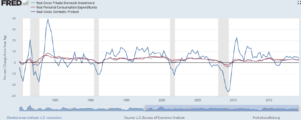
Investment is highly volatile, which is around 3-4% more volatile than GDP. Small changes in GDP usually cause big changes in Investment.
  投资是高度地波动的，比国内生产总值的波动性大3-4%。国民生产总值中的微小的改变通常会导致投资中的巨大变化。

2. Some empirical facts on investments

  投资上的一些经验事实

These statistics are for the whole aggregate economy. To properly understand the behavior and determinants of aggregate investment, we need to study investment at the firm/business level.
  这些统计数据是针对整个总体的经济。为了正确理解总投资的行为和决定因素，我们需要研究企业/商业层面的投资。

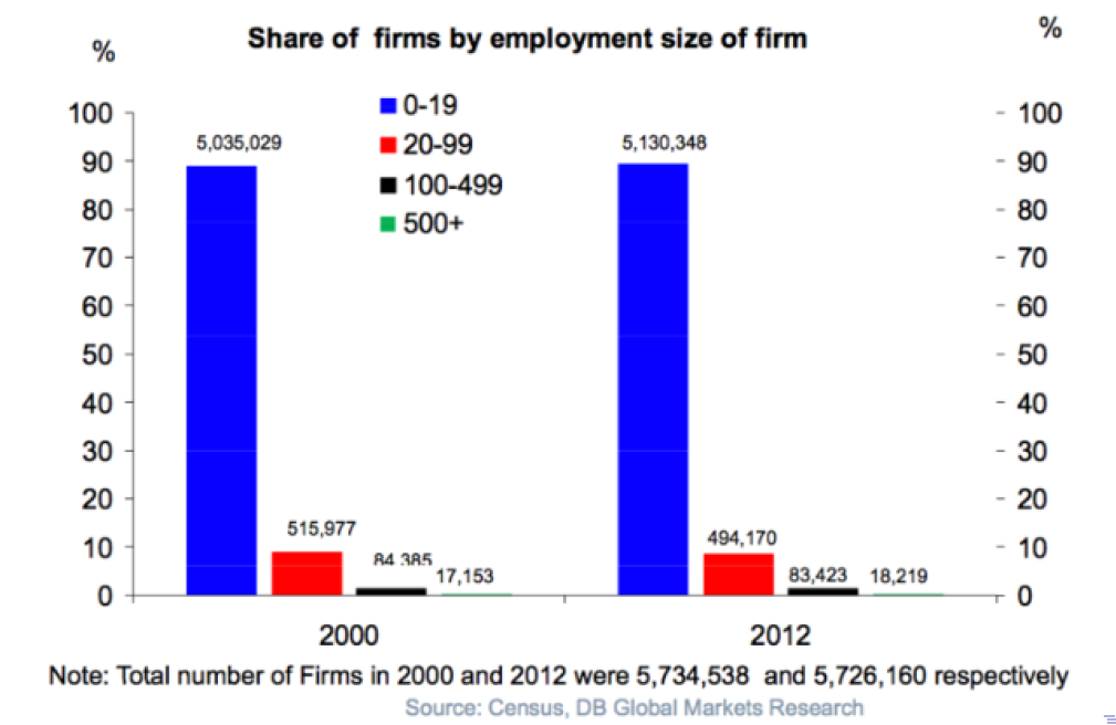
Accoding to the Census from DB Global Markets Research, the total number of firms (public + private) in the US is around 5-6 million. 90% of these firms have less than 20 employees. Besides, the number of public listed firms have been declining while substantial entry and exit of firms.
  根据DB Global Markets Research的普查，美国的（公立和私立的）公司的总数大约是500-600万。百分之九十的拥有不足20名员工。此外，上市公司的数量一直在下降，而大量的公司上市和退市。

3. How do firms choose Investment?

  公司如何选择投资？

Investment has both benefits and costs. Benefits are that more investment means more capital and more capital means more production and profits. The cost of buying and using new capital cannot be ignored. Optimal Investment shoud therefore compare the marginal benefit of new capital vesus the marginal cost of installing this capital.
  投资有收益也有成本。收益是指越多的投资意味着越多的资本，越多的资本意味着越多的生产和利润。购买和使用新资本的成本也不可以忽视。因此，最优的投资应将新资本的边际效益与安置该资本的边际成本相比较。

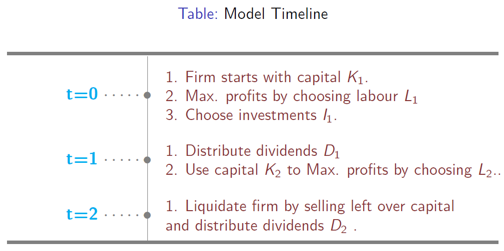
We will start with a two-period investment model. Consider the problem of a firm that lives for only two periods. The firm starts with capital \(K_1\) in the beginning of period 1 and it has to decide on how much to invest in period 1.
  我们将从一个连个周期的投资模型开始。我们将从两个时期的投资模式开始。考虑一个只存在两个时期的公司的问题。公司在第1期的开始时从资本 \(K_1\) 开始，它必须决定在第1期投资多少。

The cost of \(I_1\) units of investments is \(P_1^K\) · \(I_1\), where \(P_1^K\) is the price of a unit of capital. The stock of capital in the second period depends on the depreciation rate \(\delta\) and the level of investments today \(I_1\).
   \(I_1\) 单位的投资的成本是 \(P_1^K\) · \(I_1\)，其中 \(P_1^K\) 是单位资本的价格。第二阶段的资本存量取决于折旧率 \(\delta\) 和当前投资水平 \(I_1\)。

The second period capital is given by:
  第二期的资本可以被给出：

\[K_2 = (1 - \delta)K_1 + I_1 \tag{1} \label{capital_accumulation}\]

The timing should be read as follows:
  这些时间点应该像下列被阅读：

1. \(t = 0\) is beginning of period 1, 阶段1的开始，
2. \(t = 1\) is end of period 1 or beginning of period 2, and 阶段1的结束或阶段2的开始，以及
3. \(t = 2\) is end of period 2. 阶段2的结束。

Investment has one period delay, that is, if you choose \(I\) units of investment now, you can use it for production only in the next period. The value of the firm is maximized at \(t = 0\), which means future period values should be discounted to present value.
  投资有一个时期的延迟，也就是说，如果你现在选择 \(I\) 个投资的单位，你只能在下一个时期将其用于生产。公司的价值在 \(t=0\) 时刻最大化， 这意味着未来期间的价值应该折算为现在的价值（现值）。

An amount of money today is worth more than the same amount in the future. 1$ today is worth \((1 + r )\)$ one period from now and \((1 + r )^2\)$ two periods from now, where \(r\) is the interest rate. Present Value is the current value of a future sum of money or stream of cash ows given some return. In general,
  今天的钱比将来的钱值钱多了。今天的1美元在距今的一个周期后值 \((1+r)^2 \)美元，而且在距今的两个周期后值 \((1+r) \)美元，这里的 \(r \) 是利率。 现值是指在一定回报率下，一笔资金或者现金流的未来总额的现在的价值。一般来说，

\[\text{Present Value} = \frac{\text{Future Value}}{(1+r)^2} \ ,\]

  where \(r\) is the interest rate of return and \(n\) is the number of periods.
  在这里的 \(r\) 是回报的利率而 \(n\) 是周期数。

The firm then uses this capital for production in period 2 and at the end of the period sells off the remaining capital at price \(P^K_2\) . The operating profit made by the firm each period is given by:
  然后，这个公司在第二阶段将这些资本用于生产， 并在该阶段的末尾以 \(P^K_2\) 这一价格出售剩余资本。公司每个时期的营业利润由以下公式得出：

\[\pi(K_i)=\max_{L} \{ F(K,L) - wL \},\ where\ i = \{1,2\} \ , \tag{2} \label{operatingProfit}\]

where you are maximizing revenue net of labor costs given by the wage, \(w\), times \(L\) the labor units. function \(F(.)\) is the production function that is concave and it represents the total output produced by the firm using both capital and labor inputs. By assuming that the price of output is one, this is also the revenue.
  当你在最大化收入，人力成本为平均工资 \(w\) 乘以 劳动单位\(L\)。这个函数是凹的生产函数（译者注：中国大陆数学界某些机构关于函数凹凸性定义和国外的定义是相反的。Convex Function在某些中国大陆的数学书中指凹函数。Concave Function指凸函数。但在中国大陆涉及经济学的很多书中，凹凸性的提法和其他国家的提法是一致的，也就是和数学教材是反的。举个例子，同济大学高等数学教材对函数的凹凸性定义与本条目相反，本条目的凹凸性是指其上方图是凹集或凸集，而同济大学高等数学教材则是指其下方图是凹集或凸集，两者定义正好相反。），它企业使用资本和劳动力投入所产生的总产出。假设产出的价格是1，这也是收入。

A production function is a technology that transforms inputs to output.
  生产函数代表的是一种将投入转换为产出的技术。

\[Output = f(Input_1, Input_2, ...Input_n).\]

An example is a Cobb-Douglas production funciton:
  例如，柯布-道格拉斯生产函数：

\[f(K,L)=K^\alpha L^{1-\alpha}\ ,\]

  where \(\alpha\) is a parameter that usually takes the value 1/3.
  其中 \(\alpha\) 是一个通常取值为1/3的参数。

First derivative with respect to inputs is called the marginal product:
与投入有关的一阶导数称为边际产品：

\[\text{Marginal Product of Capital} (MPK) = \frac{\partial f(K,L)}{\partial K}\] \[\text{Marginal Product of Labor} (MPL) = \frac{\partial f(K,L)}{\partial L}\]

   Note: Operating profits is the maximum value given by the solution to eq. \eqref{operatingProfit}.
   注意： 营业利润是等式 \eqref{operatingProfit} 的解给出的最大值。

For this, we need to take the First-Order Condition (FOC) with reference to (w.r.t or WRT) \(L_i\):
  为此，我们需要去求得关于 \(L_i\) 的最佳化条件（译者注：即对生产函数关于劳动单位的数量这一未知量求取一阶导数为0时的均衡解）。

\[\frac{\partial F(K_i,\ L_i)}{\partial L_i} - w = 0\]

Optimal units of labor is such that the marginal product of labor equals the wage rate. The solution of this FOC gives us our optimal labor \(L_i^*\). The value of profits at \(L_i^*\) gives us the maximum value of profis, \(\pi(K_i)\) for both periods \(i = 1, 2\).
  最佳劳动单位是指劳动的边际产出等于工资率。这个FOC的解给出了我们的最优的劳动数量 \(L_i^*\)。利润在 \(L_i^*\) 时的价值给出了两个时期 ( \(i=1，2\) )的利润最大值 \(\pi(K_i)\) 。

All profits left after accounting for costs are distributed as dividends to the shareholders. Dividend at each period is given by the operating profits net of investment costs. Dividends for period 1 is:
  核算成本后剩下的所有利润都作为股息分配给股东。每一期的股息按扣除投资成本后的营业利润计算。第1期的股息为：

\[D_1 = \pi(K_1) - I_1 P^K_1 \tag{3}\label{divident1}\]

and for period 2 is given by:
  以及第二期的为：

\[D_2 = \pi(K_2) - I_2 P^K_2\]

  as the firm sells off any left over capital at the end of period 2. Note: The firm only lives for two periods, so capital at time 3 is zero:
  因为公司在第二期的结束时售卖完所有剩余的资产。注意：公司只维持了两个阶段，所以第三个阶段的资产数为0。

\[\because\ K_3 = (1-\delta) K_2 + I_2 = 0\] \[\implies\ I_2 = -\ (1-\delta) K_2\]

  Take \( I_2 = -\ (1-\delta) K_2 \) in the above equation into eq. \( D_2 =\pi(K_2) -I_2 P^K_2 \) , now dividends at time 2 is given by:
  将上面的等式中的\( I_2 ( = -\ (1-\delta) K_2 ) \)代入第二期分红的等式中，第二阶段的分红可以转化为：

\[\begin{align} \therefore\ D_2 & = \pi(K_2) -I_2 P^K_2 \\\\ & = \pi(K_2) + (1 - \delta) P^K_2 K_2 \\\\ \end{align} \tag{4} \label{divident2}\]

The main objective of the firm is to maximize the shareholder wealth or in other words, the present discounted sum of dividends:
  公司的主要目的是最大化股东的财富，或者换句话说，当前的股息的贴现总额。

\[\max_{I_1} \left ( D_1 + \frac{1}{1+r} D_2 \right ) \tag{5} \label{discountedSum1}\]

The discounting is done using the real interest rate, \(r\) . We need to discount as dividends received in the future is worth less than current dividends. Substitute \(D_1\), \(D_2\) with eq. \eqref{divident1}, \eqref{divident2} here, eq. \eqref{discountedSum1} can be rewritten as:
  贴现是用实际利率 \(r\) 进行的。我们需要贴现，因为收到的股息价值低于当前股息。将这里的等式\eqref{divident1}, \eqref{divident2}的\(D_1\), \(D_2\)，等式 \eqref{discountedSum1} 可以被改写为：

\[\max_{I_1} \left ( \pi(K_1) - I_1 P^K_1 + \frac{1}{1+r} \left [ \pi(K_2) + (1 - \delta) P^K_2 K_2 \right ] \right ) \tag{6} \label{discountedSum2}\]

To solve this optimization problem, substitute \(K_2\) from eq. \eqref{capital_accumulation} \(K_2 = (1 - \delta)K_1 + I_1 \) in eq. \eqref{discountedSum2}:
  若要解决此优化问题，请用公式 \eqref{capital_accumulation} \(K_2 (= (1 - \delta)K_1 + I_1 ) \) 的用来替代 \(K_2 \)。

\[\max_{I_1} \left ( \pi(K_1) - I_1 P^K_1 + \frac{1}{1+r} \left [ \pi ( (1 - \delta) K_1 + I_1 ) + (1 - \delta) P^K_2 ( (1 - \delta) K_1 + I_1) \right ] \right ) \tag{7} \label{discountedSum3}\]

Now take the derivative w.r.t \(I_1\) to eq. \eqref{discountedSum3} and equate it to zero:
  现在求取等式\eqref{discountedSum3}关于\(I_1\) 的导数的，并将其导数式等于0：

\[-\ P^K_1 + \frac{1}{1+r} \left( \frac {\partial \pi(K_2)} {\partial I_2} + (1 - \delta) P^K_2 \right) = 0\]

  Note that \(\pi (K_2)\) is an implicit function of investment, so we have to use the chain rule.
  注意\(\pi (K_2)\)是一个隐含的投资函数，所以我们必须使用链式法则。

\[\frac{\partial \pi(K_2)}{\partial I_1} = \frac{\partial \pi(K_2)}{\partial K_2} \frac{\partial K_2}{\partial I_1} = \frac{\partial \pi(K_2)}{\partial K_2} · \frac{\partial ((1 - \delta)K_1 + I_1)}{\partial I_1} = \frac{\partial \pi(K_2)}{\partial K_2} · (1) \tag{8} \label{derivative}\]

We denote the partial derivative w.r.t capital \(\pi_K(K_2)\) as \(\frac{\partial \pi(K_2)}{\partial K_2} \), which is the marginal product of capital. To solve this optimization problem , we need to get the first order condition. The first order condition (F.O.C) with respect to investment at time 1, \(I_1\), the eq. \eqref{derivative} can be rewrited as:
  我们将关于资本的偏导数 \(\pi_K(K_2)\)表示为 \(\frac{\partial \pi(K_2)}{\partial K_2} \)，这是资本的边际生产量。

\[P^K_1 = \frac{1}{1+r} \left ( \pi_K(K_2) + (1 - \delta) P^K_2 \right) \tag{9} \label{price1}\]

   or:

\[\pi_K(K_2) = (1+r) P^K_1 - (1 - \delta) P^K_2 \tag{10} \label{partialDerivative}\]

A firm should invest in capital until the value of the extra output that capital produces falls to equal the user cost. That is:
  一个公司应该继续向资本中投资，直到这一份的资本产出的额外的产出值下落到等于资产的使用成本，那就是：

\[\text{Marginal Product of Capital}\ (MPK)\ =\ \text{User Cost of Capital} \tag{11} \label{MPKuserCost}\]

The left-hand side is the marginal profitability of capital; due to law of diminishing returns ( \(F\) is concave), it is decreasing in \(K_2\).
  左手边是资本的边际利润，由于收益递减规律（F是凹函数），它在 \(K_2\) 上递减。

The right-hand side is what is called the user cost of capital, and reflects the total cost to hiring one more unit of capital in period 2. It depends on the interest rate \(r\), the depreciation rate \(\delta\), and the price of capital today (when you buy it) and tomorrow (when you sell it).
  右手侧是被叫做资本的使用成本，反映了阶段2中租借一个更多单位的资本的总成本。 它依赖于利率 \(r\)，折旧率 \( \delta \), 以及今日资本价格（当你购买它时）与明日的（当你卖出它时）。

Special Case: If the price of capital is constant \(P^K_1 = P^K_2 = P^K \), then:
  特例：如果资本的价格时恒定的 \( (P^K_1 = P^K_2 = P^K) \)，则：

\[\pi_K(K_2) = (r + \delta) P^K \tag{13} \label{specialCase}\]

The cost of using one unit of capital \(\pi_K(K_2)\) is the loss of interest foregone by buying a machine instead of saving the money \(r P^K\), plus the depreciation (maintenance) cost of capital \(\delta P^K\).
  使用一个单位的资本去购买机器而不是存款，其成本 \(\pi_K(K_2)\) 是利息的放弃的损失 \(r P^K\)，加上资产的折旧（维护）费用 \(\delta P^K\)。

Optimal investment decisions can also be reasoned by no arbitrage condition.
  最优的投资决策也可以被无套利条件来推理。

No Arbitrage: If an investor is maximizing profits, then the two investments must yield the same return. Why? Consider an investor faced with two different investment projects. If one of the projects yielded a higher return, then the investor would not be maximing profits since he/she can always allocate more investment towards the high return activity and get more profits.
无套现：如果一个投资者正在最大化利润，那么这两个投资必须产生相同的回报。为什么？假设一个投资者面临两个不同的投资项目。如果其中一个项目产生了更高的回报，那么投资者就不会实现利润最大化，因为他/她总是可以将更多的投资用于高回报活动，从而获得更多的利润。

In our model, the firm manager had two options:
  在我们的模型中，公司的管理者有两种选择：

1. Invest one unit of capital and get returns given by the
      1. 投资一个单位的资本并获取下面的计算过程所得到的回报： \[ \text{Marginal Product of Capital} + \text{Capital Gains} - \text{Depreciation Cost} \]
2. Not Invest and get returns by depositing the money in the bank.
      2. 不投资而通过将钱存入银行取得的回报

For profit maximization, both activities should yield the same return by no arbitrage condition. Rearranging gives us the same solution as in eq. \eqref{partialDerivative}.
  为了利润最大化，两种活动应该在无套现的情况下产生相同的回报。重新的安排会给我们与等式 \eqref{partialDerivative}相同的解答。

\[\underbrace{r P^K_1}_{\text{Net Return from Bank}} = MPK + \underbrace{(P^K_2 - P^K_1)}_{\text{Capital Gains}} - \underbrace{ \delta P^K_2}_{\text{Depreciation Cost}}\]

Aritrage arguments can also be used as a way to easily understand the impact of policies on investment.
  算术论证也可以作为一种容易地去理解政策对投资的影响的方法。

Example: How does an increase in the corporate tax rate impact investment?
  例子：企业税率的提高对投资有何影响？

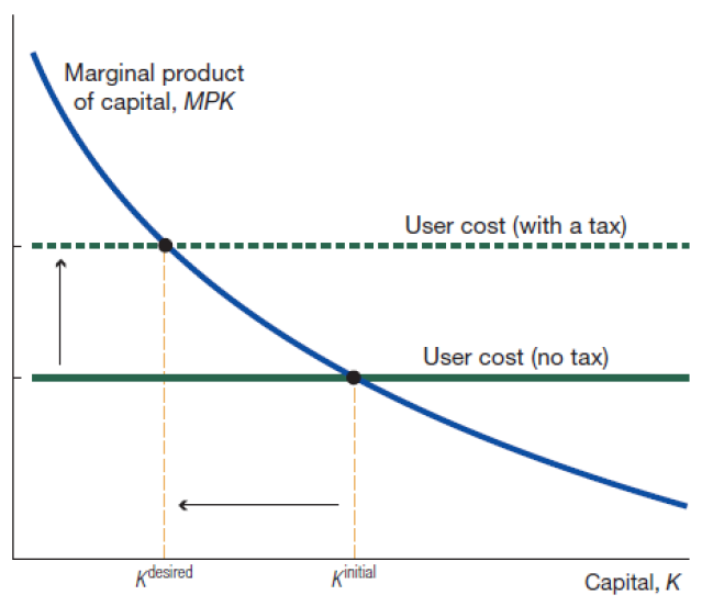
An increase in tax rate means that the firm has to pay an additional amount as taxes from its marginal product of capital. Denoting the tax rate by \( \tau \) , the no arbitrage condition can be written as:
  税率的提高意味着公司必须从其边际资本产出中支付额外的税款。以 \( \tau \) 表示税率，无套利条件可写为：

\[r P^K_1 = \underbrace{(1-\tau)MPK}_{\text{Net Return after taxes}} + (P^K_2 - P^K_1) - \delta P^K_2\]

The tax rate essentially increases the user cost of capital.
  税率实质上增加了资金的使用成本。

\[MPK = \frac{r P^K_1 - (P^K_2 - P^K_1) + \delta P^K_2} {1- \tau}\]

This model is also called the user cost model and is useful to understand long-run capital accumulation and the effect of tax policies but abstracts from many realistic features.
  这个模型也被称为用户成本模型，它有助于理解长期资本积累和税收政策的效果，但它抽象了许多现实特征。

An implication of the model is that the capital stock will adjust very quickly whenever \(r\) or \(\delta \) change. In other words, this model predicts that investment will be very smooth contradicting the data. If there are no costs of building a factory, then even infinite rates of investments is theoretically possible!
  该模型的一个含义是，无论何时 \(r\) 或 \(\delta \) 发生变化，资本存量都会迅速调整。换句话说，这个模型预测投资将非常平稳，与数据相矛盾。如果没有建厂的成本，那么即使是无限的投资率在理论上也是可能的！

In reality firms do not respond so fast because there are impediments to adjustment. Furthermore, decision of the firm are not static but forward looking.
  事实上，由于存在调整的障碍，企业的反应不会那么快。此外，公司的决策不是静态的，而是前瞻性的。

Current investment decisions are also based on expectations of future profits. Firms’ expand their capital stocks when they expect their sales to grow and cost of capital to be low and contract them when when they expext their sales to fall and the cost of capital to be high.
  目前的投资决策也是基于对未来利润的 预期。当企业期望销售额增长、资本成本较低时，它们会扩大资本存量；当预期销售额下降、资本成本较高时，它们就会收缩资本存量。

These facts motivated the development of the adjustment cost model, also known as Tobin's Q model which is the benchmark model in this literature.
  这些事实推动了调整成本模型的发展，也就是本文（注：应该是老师用的参考书）中的基准模型Tobin’s Q模型。