translated by damien from sildes of Sisi Ramanan

Unit 4 Testing Q

1. Investment Q Model

This model predicts that investment and Q are related. Knowing Q is sufficient to predict what the investment level will be. Is Q readily observable in the data?
  该模型预测投资与Q值相关。 知道Q值就足以预测投资水平。 Q在数据中容易观察到吗？

Remember Q is given by,
  记住Q是由， \[Q = \beta E[V _{K’} (\theta ‘, K’)] \] the derivative of the value function, hence called Marginal Q. To test Q theory, we need to measure this value. The marginal value is unobservable making empirical testing of investment Q models extremely difficult.
  值函数的导数，因此称为边际Q。 为了检验Q理论，我们需要测量这个值。 边际价值是不可观察的，这使得投资Q模型的实证检验非常困难。

As the value function and hence its derivative is not observable, testing adjustment cost investment model is difficult. We need to find a suitable proxy for the derivative of the value function. A good proxy is to substitute the marginal value of the firm with its average value. Under what conditions is the average value a good proxy for the marginal value?
  由于价值函数及其导数是不可观测的，因此很难检验调整成本投资模型。我们需要为值函数的导数找到一个合适的代理。一个好的代理是用企业的平均价值代替企业的边际价值。在什么条件下，平均值能很好地代表边际价值？

2. Hayashi’s Result

Hayashi (1982) established some conditions under which the average and marginal Q coincide.
  Hayashi（1982）建立了一些条件，在这些条件下，平均Q和边际Q是一致的。

Proposition

Hayashi showed that a firm’s marginal Q equals average Q when the following three conditions are satisfied:
  Hayashi指出，当满足以下三个条件时，公司的边际Q等于平均Q：

1. The firm is a price taker in the output market.
     一, 这家公司是输出市场的价格接受者。
2. Production function is linearly homogenous.
     二， 生产函数是线性齐次的。
3. Cost functions are linearly homogenous.
     三， 成本函数是线性齐次的。

The first condition says that the firm is operating in a perfectly competitive environment such that it has no power in the pricing of its output product. The market determines the product price.
  第一个条件是，公司在一个完全竞争的环境中经营，因此它没有权力对其产出产品定价。市场决定产品价格。

Linear homogeneity means homogenous functions of order one. A production function which is homogenous of degree one displays constant returns to scale. Note: Refer to Marginal and Average q.pdf on Moodle for more on this.
  线性齐次是指一阶齐次函数。 一个一级同质的生产函数显示出恒定的规模收益。 注：请参阅Moodle上的Marginal and Average q.pdf了解更多信息。

Hayashi’s results form the basis of empirically implementing the investment Q model and facilitates its testing. We can now substitute the unobservable marginal Q with the observable average Q.
  Hayashi的结果构成了实证实施投资Q模型的基础，并有助于其测试。 我们现在可以用可观测的平均Q代替不可观测边际Q。

That is,
  那就是，

\[\text{Marginal Q} = E [V _{K'}(θ', K')] = \frac{V}{K} = \text{Average Q}\]

3. Empirical Testing

Tests of Q theory on panel data are frequently conducted using the following empirical specification:
  对面板数据的Q理论测试通常使用以下经验规范进行：

\[I _{it} / K _{it} = a _0 + a_1 Q _{it} + a_2 X _{it} + \epsilon _{it} \tag{1} \label{empiricalSpecification}\]

 This is a panel regression, where the subscript \(i\) denotes the individual firm (or plant) and \(t\) denotes time. We are regressing investment rate \(I/K \) on \(Q\) and some control(s) \(X\). What is the role of these controls \(X _{it}\) ?
  这是一个面板回归，其中下标 \(i\) 表示单个公司（或工厂），而 \(t\) 表示时间。 我们正在回归投资率 \(I/K \) 对 \(Q\) 和一些控制 \(X\)。 这些控件的作用是什么？

Q theory says that the value of Q is sufficient to incorporate all relevant information related to production and investment. That is, no other variable should impact investment. These variables \(X _{it}\) are included as a means of testing the theory, where the theory predicts that these variables from the information set should be insignificant. In other words, the coefficient \(a _2\) should be statistically insignificant.
  Q理论认为Q值足以包含所有与生产和投资相关的信息。也就是说，没有其他变量会影响投资。 这些变量 \(X _{it}\) 作为测试理论的一种手段被包括在内，理论预测这些来自信息集的变量应该是无关紧要的。 换言之，系数 \(a _2\) 在统计学上是不重要的。

The estimate of the coefficient \( \hat{a} _1\) also provides information on the adjustment cost paramter. This comes from a modification of the adjustment costs to the form:
  系数 \( \hat{a} _1\) 的估计也提供了调整成本参数的信息。 这源于调整成本的形式：

\[C (K', K ) = \frac{\phi}{2} \left ( \frac{K' − (1 − \delta K)}{K} − a _i \right )\]

We will focus on three seminal papers in the investment literature - Fazzari, Hubbard, Petersen (1988), Gilchrist and Himmelberg (1995) and Cooper and Ejarque (2003). These papers make use of Hayashi’s proposition and test the Q theory of investment.
  我们将重点关注投资文献中的三篇开创性论文——Fazzari、Hubbard、Petersen（1988）、Gilchrist和Himmelberg（1995）以及Cooper和Ejarque（2003）。 这些论文利用了林氏的命题，对投资的Q理论进行了检验。

Question: Can investment be entirely explained by average Q?
   问题：投资能否完全用平均Q来解释？

1. If yes, then this validates the Q model of investment.
     一，如果是，那么这就验证了投资的Q模型。
2. If no, what other variables are important in explaining firm level investment?
     二，如果没有，在解释公司层面的投资时，还有哪些变量是重要的？

4. FHP 1988

– Empirical Implementation of Q Model - Fazzaari, Hubbard, Petersen (1988)

We will start with the paper by Fazzari, Hubbard, Petersen (1988). FHP postulate a regression of the form:
  我们将从Fazzari，Hubbard，Petersen（1988）的论文开始。 FHP假设回归形式：

\[I _{it} / K _{it} = a _0 + a_1 Q _{it} + a_2 (CF _{it} / K _{it}) + \epsilon _{it} \tag{2} \label{es2}\]

 where the investment rate is regressed on average Q and a control given by cashflow over capital.
  其中投资率是回归的平均Q和现金流对资本的控制。

The idea is that if there are financial constraints (or capital market imperfections), then these will be felt more at firms that are either unable to find it or difficult to obtain at a reasonable cost.
  这个想法是，如果存在财务约束（或资本市场不完善），那么那些要么找不到，要么很难以合理成本获得的公司，会更容易感受到这些限制。

If their idea is true, then investment for financially constrained firms will depend on variables other than Q. Testing the coefficient \(a _2\) might provide evidence for this conjecture. The control variable suggested by FHP is cash-flow.
  如果他们的想法是真的，那么对财务拮据的公司的投资将取决于除Q以外的其他变量。 测试系数 \(a _2\) 可能会为这个猜想提供证据。 FHP提出的控制变量是现金流量。

They classify firms into three groups:
  他们把公司分为三类：

1. Class 1: Dividends/Income < 0.1
     一，第1类：股息/收入<0.1
2. Class 2: 0.1 < Dividends/Income < 0.2
     二，第2类：0.1<股息/收入<0.2
3. Class 3: All other firms.
     三，第3类：所有其他公司。

Data:
  数据：

1. Value Line, US firms
     一，价值线，美国公司
2. Time period: 1970-1984
     二，时间：1970-1984
3. Manufacturing Sector
     三，制造业

Measuring Q:
  测量Q：

1. Q at the beginning of the period
     一，期初Q
2. Ratio of market value (value of equity plus value of debt) over replacement value of capital.
     二，债务（资本）重置价值超过市场价值的比率。

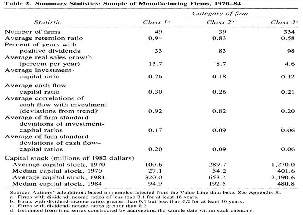
The summary table suggests the following:
  汇总表建议如下：

1. Firms in class 1 and 2 have retained most of their income in the majority of years.
     一，一级和二级的公司在大多数年份里保留了大部分收入。
2. Are relatively small.
     二，相对较小。
3. Have experience most growth in their capital stock.
     三，经历了最快的资本存量的增长。
4. Exhaust almost all of their cash flow in their investment.
     四，几乎耗尽了他们投资的现金流。
5. They also exhibit a much higher correlation of investment to cash flow.
     五，它们还表现出投资与现金流之间更高的相关性。

5. Results and Issues

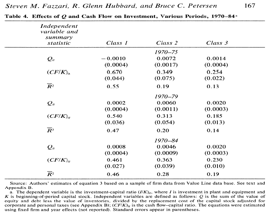
More financially constrained firms (Class 1) exhibit significantly greater investment cash flow sensitivities than firms that appear less financially constrained. Difference in cash flow coefficients between different classes of firms are always statistically significant. \(R^2\) is always higher for these firms.
  财务状况较差的公司（1类）比财务状况较差的公司表现出更大的投资现金流敏感性。 不同类别企业的现金流量系数差异在统计学上总是显著的。 \(R^2\) 对这些公司来说总是更高。

These results are robust to a number of checks:
  这些结果对许多检查是可靠的：

1. Possible measurement errors in Q.
     一，Q中可能的测量误差。
2. Using lagged values (last period for instance) of Q and \(CF/K\).
     二，使用Q和 \(CF/K\) 的滞后值（例如最后一个时段）。
3. Using end of period Q.   三，使用期末Q。
4. Alternate measurement of Q by using sales.   四，用销售额替代Q值。
5. Results are consistent across different industries.   五，不同行业的结果是一致的。

Possible issues with their approach:
  他们的方法可能存在的问题：

1. Q may not be accurately reflecting market fundamentals due to excessive volatility in equity market.
     一，由于股市波动过大，Q可能无法准确反映市场基本面。
2. Measurement errors in Q could be correlated with cash flow.
     二，Q的计量误差可能与现金流量有关。
3. Cash flow may reflect news about future profitability of investment that is not captured by beginning of period Q.
     三，现金流可能反映了有关投资未来盈利能力的新闻，而这些新闻并没有在第Q期初得到反映。