Unit 5 Multi Period Market Model

多期市场模型

Overview

• One-period models
  • Elementary market model
  • Single-period market model
• Multi-period market model
  • Role of Information
  • Can we ‘split’ into many single-period models?

Elementary Market Model

• 2 states of nature
• 2 assets: riskless bank account (governemnt bond) and an ‘underlying asset’ - risky share
• The aim is to replicate particular contingent claim: form a portfolio of two assets which will give you exactly the same payoff as the contingent claim.
• Important notions are introduced
  • arbitrage
  • risk neutral probability measure (RNPM)
• We show that the replicating strategy (portfolio weights) is fully explained by RNPM
• In the elementary model there is a simple formula to compute RNPM.
• If there is no arbitrage you can always find RNPM and construct replicating strategy.
  • you can guess this is because there are two states of nature and two assets

  Single-Period Market Model

• \(K \geq 2\) states of nature. We work with finite K.
• \(N \geq 2\) risky assets and one riskless bank account (governemnt bond). So N + 1 securities in portfolio.
• The aim is the same: replicate particular contingent claim by forming a portfolio of assets which will give you exactly the same payoff as the contingent claim. Important notions are introduced.
  • arbitrage
  • risk neutral probability measure (RNPM)
  • complete market model
  • attainable claim
• FATP: Model \(\cal M\) is arbitrage free \((\Leftrightarrow)\)at least one RNPM exists.
  • Need a procedure to find RNPM. If we can construct a RNPM then there is no arbitrage. We discussed the procedure.
  • If we know RNPM we can use it to construct the replicating strategy.
  • If we have a replicating strategy then the contingent claim is attainable.
• Complete market: all contingent claims are attainable.
• Need to have at least as many (different) securities (N + 1) as (different) states of nature (K).
• So, we are naturally interested in working with complete markets. There is a unique RNPM there. And we learned how to construct a replicating portfolio and so we learned how to find an arbitrage price of a contingent claim.
• However, when markets are incomplete, then certain claims can still be attainable.

### Multi-Period Market Model

• Many (possibly infinite number of) periods.
• \(K \geq 2\) states of nature.
• \(N \geq 2\) risky assets and one riskless bank account (governemnt bond). So N + 1 securities in portfolio.
• Unlike in single-period models, information at each period changes.
• We discussed ho to model the information set (partitions and filtrations). When computing expectations at period t they are now conditional on ‘information available at time t’, not ‘the whole information’.

Outline We will examine the following issues:
1 Trading Strategies and Arbitrage-Free Models
2 Risk-Neutral Probability Measures and Martingales
3 Fundamental Theorem of Asset Pricing
4 Arbitrage Pricing of Attainable Claims
5 Risk-Neutral Valuation of Non-Attainable Claims
6 Completeness of Multi-Period Market Models

1 Trading Strategies and Arbitrage-Free Models

Primary Traded Assets

To specify a multi-period market model \(\cal M= (B, S^1, . . . , S^n)\) we have to examine the concept of a dynamic trading strategy and the associated wealth process. We first define primary traded assets

• Let r be the interest rate. The money market account is denoted by \(B_t\) for t = 0, 1,… ,T where

\(B_t = (1 + r )^t\)

• There are n risky assets, called stocks, with price processes denoted by \(S_t^j\) for t = 0, 1,…,T.
• We are given a probability space \((\Omega,\cal F,\mathbb P)\) endowed with a filtration \(\mathbb F\) generated by price processes of stocks.

Dynamic Trading Strategy and Wealth Process

A dynamic trading strategy in a multi-period market model is defined as a stochastic process \((\phi_t =\phi_t^0,\phi_t^1,…,\phi_t^n)\) for t = 0, 1, . . . ,T where:

• \(\phi_t^0\) is the number of ‘shares’ of the money market account B held at time t.
• \(\phi_t^j\)is the number of shares of the jth stock held at time t.

Definition (Value Process)

The wealth process (or value process) of a trading strategy \((\phi =\phi^0,\phi^1,…,\phi^n)\) is the stochastic process \(V (\phi)\) given by

\[V_t (\phi) = \phi_t^0 B_t + \Sigma _{j=1}^n \phi_t^j S_t^j .\]

Self-Financing Trading Strategy

Definition (Self-Financing Trading Strategy)

A trading strategy \(\phi\) is said to be self-financing strategy if for t = 0, 1, . . . ,T - 1,
\(\phi_t^0 B_{t+1} + \Sigma_{j=1}^n S_{t+1}^j = \phi_{t+1}^0 B_{t+1} + \Sigma_{j=1}^n S_{t+1}^j\)

• The LHS of (1) represents the value of the portfolio at time t + 1 before its revision, whereas the RHS represents the value at time t + 1 after the portfolio was revised.
• Condition (1) says that these two values must be equal and this means that no cash was withdrawn or added.
• For t = T - 1, both sides of (1) represent the wealth at time T, that is,\(V_T(\phi)\). We do not revise the portfolio at time T.

Gains Process

Lemma (6.1)

For any self-financing trading strategy, the wealth process can be alternatively computed by, for t = 1, . . . ,T,

\(V_t (\phi) = \phi_t^0 B_t + \Sigma_{j=1}^n \phi_{t-1}^j S_t^j\)

Proof.

The statement is an immediate consequence of formula (1).

Definition (Gains Process)

For a trading strategy \(\phi\), the gains process \(G(\phi) = (G_t (\phi))_{0 \leq t \leq T}\) is given by

\[G_t (\phi) := (V_t (\phi)) - V_0(\phi).\]

Multi-Period Market Model

Definition (Market Model)

A multi-period market model \(\cal M= (B, S^1, . . . , S^n)\) is given by the following data:

1. A probability space \((\Omega,\cal F,\mathbb P)\) endowed with a filtration \(\mathbb F= (\cal F_t)_{0 \leq t \leq T}\) .
2. The money market account B given by \(B_t = (1 + r )^t\) .
3. A number of financial assets with prices \(S^1, . . . , S^n\), which are assumed to be \(\mathbb F\)-adapted stochastic processes.
4. The class F of all self-financing trading strategies.

Increment Processes

• As in the single-period model, we define the discounted value process, gains process and discounted gains process.
• It will be convenient to use the increment processes for traded assets.

Definition (Increment Processes)

• The increment process \(\Delta S^j\) corresponding to the jth stock is deined by

\[\Delta S_{t+1}^j := S_{t+1}^j - S_t^j   for   t = 0, . . . ,T - 1\]

• The increment process \(\Delta B\) of the money market account are given by

\[\Delta B_{t+1} := B_{t+1} - B_t = (1 + r )^t r = B_t r   for   t = 0, . . . ,T - 1.\]

Discounted Processes

Definition (Discounted Processes)

The discounted stock prices are given by

\(\hat S_t^j:= \frac {S_t^j}{B_t}\) and the increments of discounted prices are \(\Delta \hat S_{t+1}^j := \hat S_t^j\). The discounted wealth process \(\hat V (\phi)\) of \(\phi\) is given by
\(\hat V_t (\phi) :=\frac {V_t(\phi)}{B_t}\)

The discounted gains process \(\hat G (\phi)\) of \(\phi\) equals

\[\hat G_t (\phi) := \hat V_t (\phi) - \hat V_0(\phi).\]

Discounted Processes

Proposition (6.1)

An \(\mathbb F\)-adapted trading strategy \(phi = (\phi_t)_{0 \leq t \leq T} \ is self-financing if and only if any of the two equivalent statements hold:

1. for every t = 1, . . . ,T

\[G_t (\phi) =\Sigma_{u=0}^{t-1} \phi_u^0 \delta G_{u+1} + \Sigma_{u=0}^{t-1} \Sigma_{j=1}^n \phi_u^j \Delta \hat S_{u+1}^j\]

1. for every t = 1, . . . ,T

\[\hat G_t (\phi) =\Sigma_{u=0}^{t-1} \Sigma_{j=1}^n \phi_u^j \Delta \hat S_{u+1}^j\]

Properties of Discounted Gains and Wealth

Proof.

[Proof of Proposition 6.1] The proof is elementary and thus it is left as an exercise.

• Note that the process \(\hat G (\phi)\) given by condition 2) does not depend on the component \(\phi^0\) of \(\phi \in \Phi\).
• In view of Proposition 6.1, the discounted wealth process of any \(\phi \in \Phi\) satifies

\[\hat V_t(\phi)=\hat V_0(\phi) + \Sigma_{u=0}^{t-1} \Sigma_{j=1}^n \phi_u^j \Delta \hat S_{u+1}^j\]

• Hence for every t = 0, . . . ,T - 1

\[\Delta \hat V_{t+1}(\phi)= \Delta \hat G_{t+1}(\phi) =\Sigma_{j=1}^n \phi_t^j \Delta \hat S_{t+1}^j\]

Arbitrage Opportunity

As usual, we work under the standing assumption that the sample space \(\Omega\) is finite (or countable).

Definition (Arbitrage Opportunity)

A trading strategy \(\phi = (\phi_t)_{0 \leq t \leq T} \) is an arbitrage opportunity if

1. \(V_0(\phi) = 0\),
2. \(V_T (\phi)(\omega) \geq\ 0 \) for all \(\omega \in \Omega\),
3. \(V_T (\phi)(w) > 0 \) for some \(\omega \in \Omega\) or, equivalently, \(\mathbb E_P(V_T (\phi)) > 0\).
   We say that a multi-period market model \(\cal M\) is arbitrage-free if no arbitrage opportunities exist in \(\Phi\).

Arbitrage Conditions

• Note that in the arbitrage conditions one can use either the discounted wealth process \(\hat V\) or the discounted gains process \(\hat G\) (instead of the wealth V).
• It is also important to note that conditions 1)-3) hold under \(\mathbb P\) whenever they are satisfied under some probability measure \(\mathbb Q\) - equivalent to \(\mathbb P\).
• The next step is to introduce the concept of a risk-neutral probability measure for a multi-period market model.
• Risk-neutral probability measures are very closely related to the question of arbitrage-free property and completeness of a multi-period market model.

2 Risk-Neutral Probability Measures and Martingales

Risk-Neutral Probability Measure

Definition (Risk-Neutral Probability Measure)

A probability measure \(\mathbb Q\) on W is called a risk-neutral probability measure for a multi-period market model \(\cal M= (B, S^1, . . . , S^n)\) whenever

1. \(\mathbb Q(\omega) > 0 \) for all \(\omega \in \Omega\),
2. \(\mathbb E_P(\Delta \hat S_{t+1}^j) | \cal F_t ) = 0\) for all j = 1, . . . , n and t = 0, . . . ,T - 1.

We denote by M the class of all risk-neutral probability measures for the market model \(\cal M\).
Observe that condition 2) is equivalent to the equality, for all

\((\mathbb E_P(\Delta \hat S_{t+1}^j) \| \cal F_t ) = \hat S_{t}^j\) The discounted stock price \(\hat S^j\) is a martingale under any risk-neutral probability measure \(\mathbb Q \in \mathbb M\).

Discounted Wealth as a Martingale

Proposition (6.2)

Let \(\phi \in \Phi\) be a trading strategy. Then the discounted wealth process \(\hat V(\phi0\) and the discounted gains process \(\hat G(\phi)\) are martingales under any risk-neutral probability measure \(\mathbb Q \in \mathbb M\).

Proof.

• Recall that \(\hat V_t(\phi)\) = \(\hat V_0(\phi)\) + \(\hat G_t(\phi)\) for every t = 0, . . . ,T,
• Since \(\hat V_0(\phi)\) (the initial endowment) is a constant, it suffices to show that the process \(\hat G_t(\phi)\ is a martingale under any \(\mathbb Q \in \mathbb M\). From Proposition 6.1, we obtain

\[\hat G_{t+1}(\phi) = \hat G_t (\phi)+ \Sigma_{j=1}^n \phi_u^j \Delta \hat S_{u+1}^j\]

Proof of Proposition 6.2

Proof. [Proof of Proposition 6.2 (Continued)]

• Hence

• We used the fact that \(\phi_t^j\) is \(\cal F_t\)-measurable and the “take out what is known” property of the conditional expectation.
• We conclude that \(\hat G (\phi)\) is a martingale under any \(\mathbb Q \in \mathbb M\).

3 Fundamental Theorem of Asset Pricing

Fundamental Theorem of Asset Pricing

• We will show that the Fundamental Theorem of Asset Pricing (FTAP) can be extended to a multi-period market model.
• Recall that the class of admissible trading strategies \(\phi\) in a multi-period market model is assumed to be the full set of all self-financing and \(\mathbb F\)-adapted trading strategies.
• It possible to show that in that case, the relationship between the existence of a risk-neutral probability measure \(\mathbb Q\) and no arbitrage for the model \(\cal M\) is “if and only if”.
• We will only prove here the following implication: Existence of \(\mathbb Q \in \mathbb M\) \(\rightarrow\) Model \(\cal M\) is arbitrage-free.

Fundamental Theorem of Asset Pricing

Theorem (FTAP)

Consider a multi-period market model \(\cal M= (B, S^1, . . . , S^n)\).
The following statements hold:

1. if the class \(\mathbb M\) of risk-neutral probability measures for \(\cal M\)is non-empty then there are no arbitrage opportunities in the class F of all self-financing trading strategies and thus the model \(\cal M\) is arbitrage-free,
2. if there are no arbitrage opportunities in the class \(\Phi\) of all self-financing trading strategies then there exists a risk-neutral probability measure for \(\cal M\), so that the class \(\mathbb M\) is non-empty.

To sum up:
Class \(\mathbb M\) is non-empty \(\Longleftrightarrow\) Market model \(\cal M\) is arbitrage-free

Proof of the FTAP \((\Longrightarrow\))

Proof.

[Proof of the FTAP \((\Longrightarrow\)) ] Let us assume that a risk-neutral probability measure \(\mathbb Q\) for \(\cal M\) exists.Our goal it to show that the model \(\cal M\) is arbitrage-free.
To this end, we argue by contradiction. Let us thus assume that there exists an arbitrage opportunity \(\phi \in \Phi\). Such a strategy would satisfy the following conditions:

1. the initial endowment \(\hat V_0(\phi) = 0\),
2. the discounted gains process \(\hat G_T (\phi) \geq 0\),
3. there exists at least one w 2 W such that \(\hat G_T (\phi)(\omega) > 0\).

On the one hand, from conditions 2. and 3. above, we deduce easily that

\[\mathbb E_P(\hat G_T (\phi)) > 0\]

Proof of the FTAP \((\Longrightarrow\)) Proof. [Proof of the FTAP (\(\Longrightarrow\))] On the other hand, using Proposition 6.1, we obtain

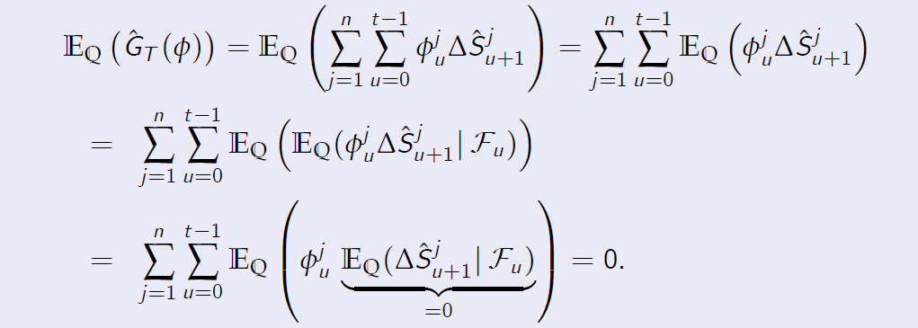
This clearly contradicts the inequality obtained in the first step. Hence there cannot be an arbitrage in the market model \(\cal M\).

Replicating Strategy

• Note that a contingent claim of European style can only be exercised at its maturity date T (as opposed to contingent claims of American style).
• A European contingent claim in a multi-period market model is an \(\cal F_T\) -measurable random variable X on \(\Omega\) to be interpreted as the payoff at the terminal date T.
  一个欧式或有债权在多期的市场模式是一种 \(\cal F_T\)-可测量的随机变量 X 在 \(\Omega\) 上解释为截止日期 T 的收益。
• For brevity, European contingent claims will also be referred to as contingent claims or simply claims.

Definition (Replicating Strategy)

A replicating strategy (or a hedging strategy) for a contingent claim X is a trading strategy \(\phi \in \Phi\) such that \(V_T(\phi) = X\), that is, the terminal wealth of the trading strategy matches the claims payoff for all \(\omega\).
或有债权 X 的复制策略（或对冲策略）是一种交易策略 \(\phi \in \Phi\)，使得 \(V_T(\phi) = X\)，即交易策略的最终财富与所有 \(\omega\)的债权收益相匹配。

Principle of No-Arbitrage

Definition (Principle of No-Arbitrage)

An F-adapted stochastic process \((\pi_t (X))_{0 \leq t \leq T}\) is a price process for the contingent claim X that complies with the principle of no-arbitrage if there is no F-adapted and self-financing arbitrage strategy in the extended model \(\cal \tilde M= (B, S^1, . . . , S^n, S^{n+1})\) with an additional asset \(S^{n+1}\) given by \(S_T^{n+1}=\pi_t X\) for \(0 \leq t \leq T-1\) and \(S_T^{n+1}=X\)

一个F-适应随机过程\((\pi_t (X))_{0 \leq t \leq T}\)是一个或有权益X的价格过程，如果扩展模型\(\cal \tilde M= (B, S^1, . . . , S^n, S^{n+1})\)中不存在 F-适应 和自筹资金的套利策略，则符合无套利原则，且附加资产\(S^{n+1}\)，由\(0 \leq t \leq T-1\)）和\(S_T^{n+1}=X\)给出。

• The standard method to price a contingent claim is to employ the replication principle, if it can be applied.
  对未定权益定价的标准方法是采用复制原则（如果适用的话
• The price will now depend on time t and thus one has to specify a whole price process \(\pi(X)\), rather than just an initial price, as in the single-period market model.
  -价格现在取决于时间t，因此必须指定一个完整的价格过程\(\pi(X)\)，而不是像单周期市场模型那样只指定一个初始价格。
• Obviously, \(\pi_T(X)=X\) for any claim X.

4 Arbitrage Pricing of Attainable Claims

Arbitrage Pricing of Attainable Claims

In the next result, we deal with an attainable claim, meaning that we assume a priori that a replicating strategy for X exists.

Proposition (6.3)

Let X be a contingent claim in an arbitrage-free multi-period market model \(\cal M\) and let \(\phi \in \Phi\) be any replicating strategy for X. Then the only price process of X that complies with the principle of no-arbitrage is the wealth process \(V (\phi)\).

• The arbitrage price at time t of an attainable claim X is unique and it is also denoted as \(\pi_t (X)\).
• Hence the equality \(\pi_t (X) = V_t (\phi)\) holds for any replicating strategy \(\phi \in \Phi\) for X.
• In particular, the price at time t = 0 is the initial endowment of any replicating strategy for X, that is, \(\pi_0 (X) = V_0 (\phi)\) for any strategy \(\phi \in \Phi\) such that \(V_T (\phi) =X\).

Example: Replication of a Digital Call Option

• The definition of hedging strategy is also used to price a contingent claim, which is called the replication principle.
• We will now examine replication of a contingent claim in a two-period market model.
• It is easy to check that this model is arbitrage-free.
  Example (6.1)
• Consider a two-period market model consisting of the savings account and one risky stock.

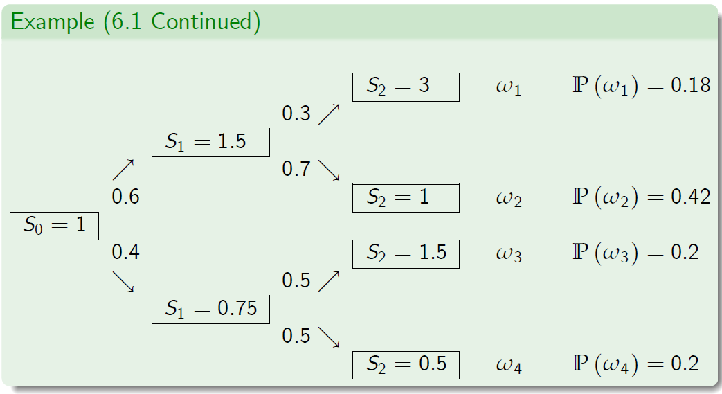
• The interest rate equals \(r=\frac{1}{9}\) so that

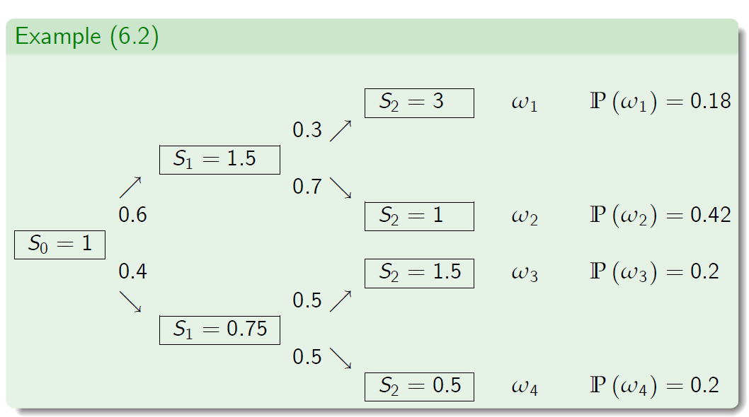
• The price of the stock is represented in the following exhibit in which the real-world probability \(\mathbb P\) is also specified.

Example: Replication of a Digital Call Option

Example (6.1 Continued)

Example: Replication of a Digital Call Option
Example (6.1 Continued)

• Consider a digital call option with the payoff function

Put another way

• By the definition of hedging strategy, we have \(V_2 (\phi) =X\) or, more explicitly,

Example: Replication of a Digital Call Option

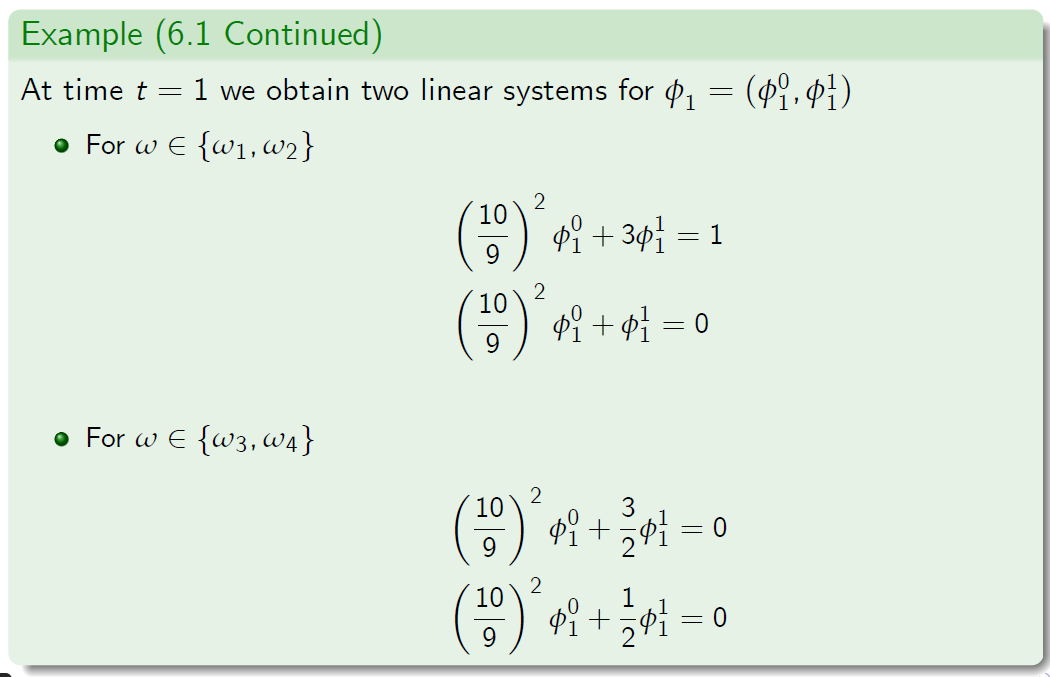
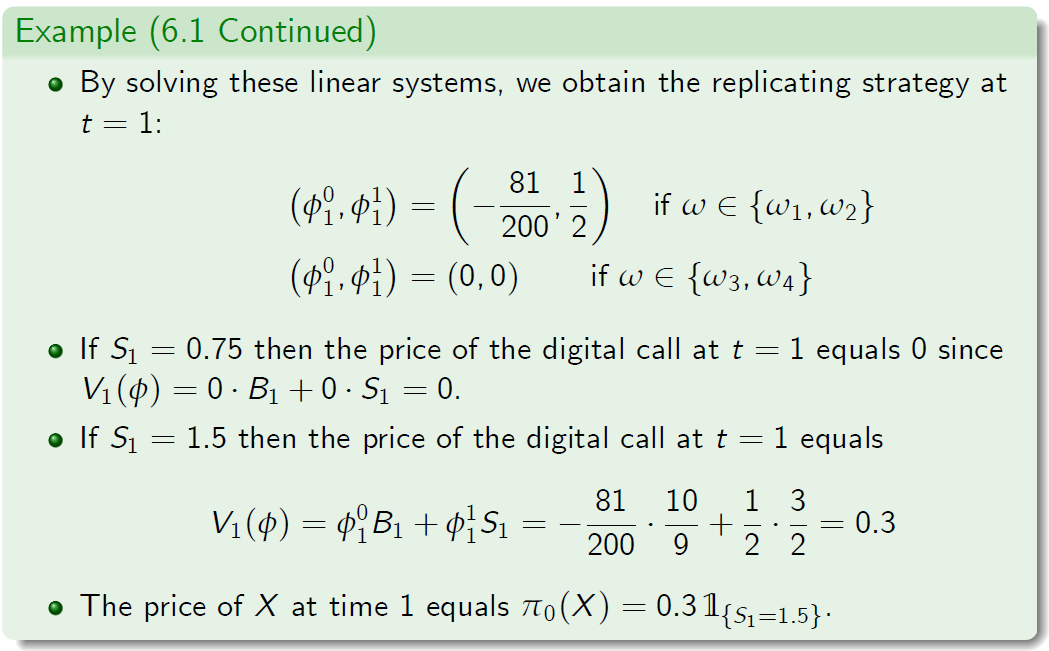
Example (6.1 Continued)

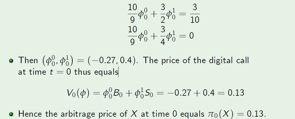
• We will now compute the price of the digital call at t = 0. The replicating strategy at time t = 0 satisfies

Example (6.1 Continued) Summary of pricing and hedging results for a digital call option.
Recall that the price at time t = 2 equals \(pi_2(X) = X\).
Replicating strategy f satisfies \(V_2(\phi) = X\).
The arbitrage price process of X equals \(\pi_(X) = V (\phi)\).

Attainability of Contingent Claims and Completeness

Definition (Attainable Contingent Claim)

A contingent claim X is called to be attainable if there exists a trading strategy \(\phi \in \Phi\), which replicates X, i.e., \(\pi_T(X)=X\).

• For attainable contingent claims, it is clear how to price them by the initial investment needed for a replicating strategy.
• As in single period market models, for some contingent claims a hedging strategy may fail to exist.

Definition (Completeness)

A multi period market model is said to be complete if and only if all contingent claims have replicating strategies. If a multi period market model is not complete, it is said to be incomplete.

5 Risk-Neutral Valuation of Non-Attainable Claims

Risk-Neutral Valuation Formula

Proposition (6.4)

Let X be a contingent claim (possibly non-attainable) and Q any risk-neutral probability measure for the multi-period market model \(\cal M\). Then the risk-neutral valuation formula

defines a price process \(\pi(X)= (\pi_t (X))_{0 \leq t \leq T}\) for X that complies with the principle of no-arbitrage.

Proof.

The proof hinges the same arguments as in the single-period case and thus it is left as an exercise. If X is attainable then can also observe that \(\hat V (\phi)\) is a martingale under \(\mathbb Q\) and apply the defiition of a martingale.

Example: Risk-Neutral Valuation

Example (6.2 Continued)

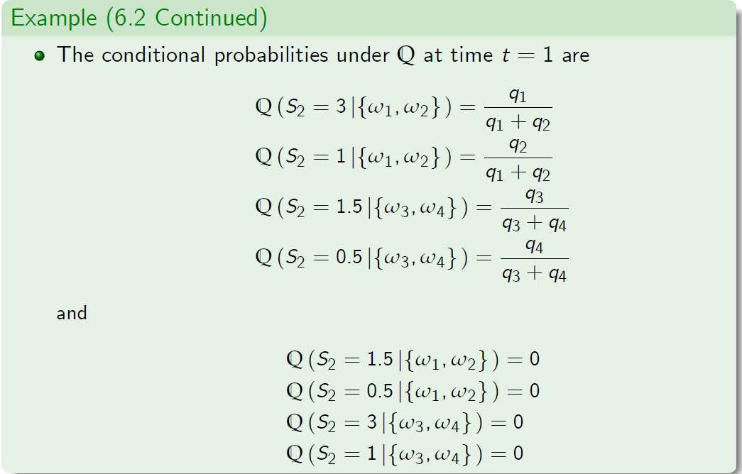
• Consider again the market model \(\cal M= (B, S)\) introduced in Example 6.1. Recall that the conditional probabilities describe the movements under the real-world probability \(\mathbb P\).
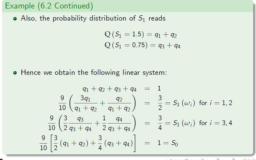
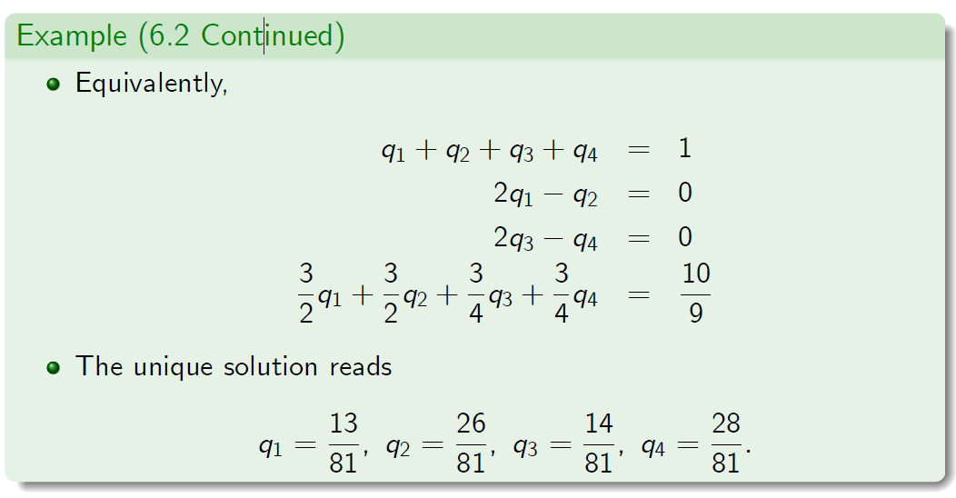
• Let \(\mathbb Q\) be a risk-neutral probability measure from M.
• We denote \(q_i = \mathbb Q (\omega_i )\) for i = 1, 2, 3, 4.
• By the definition of the risk-neutral probability, we have

Example: Risk-Neutral Valuation

Example: Risk-Neutral Probability Measure

Example: Risk-Neutral Valuation

Example: Risk-Neutral Valuation

Example (6.2 Continued)
The price of the digital call option considered in Example 6.1 can be computed as follows.

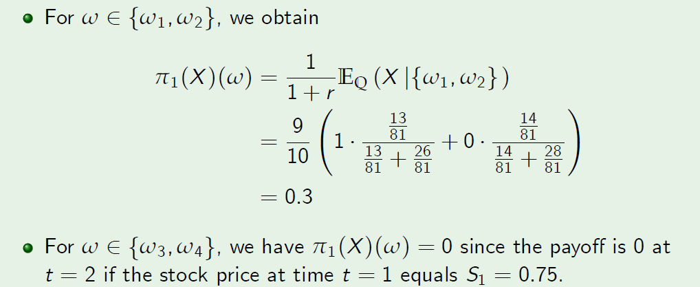
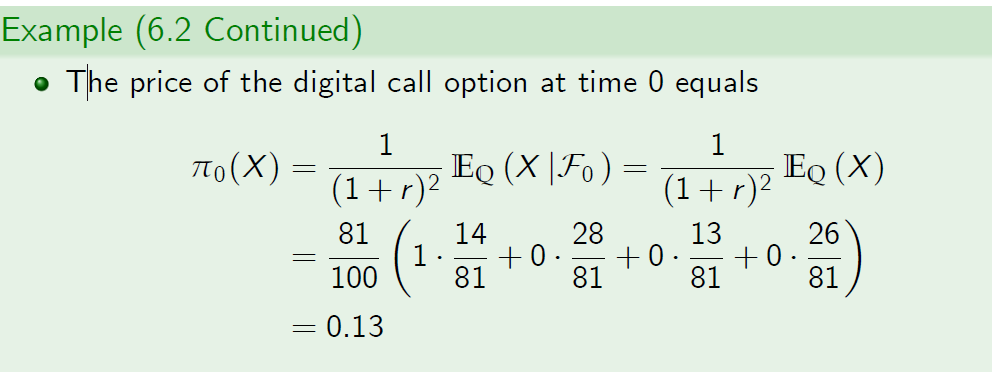
• These pricing results coincide with those obtained in Example 6.1, where we computed directly the wealth process \(V (\phi)\) of the replicating strategy \(\phi\) for X.
• As indicated earlier, a multi-period market model \(\cal M\) can be decomposed into several single-period market models.

Example: Backward Induction

Example: Backward Induction

Example (6.3 Continued)

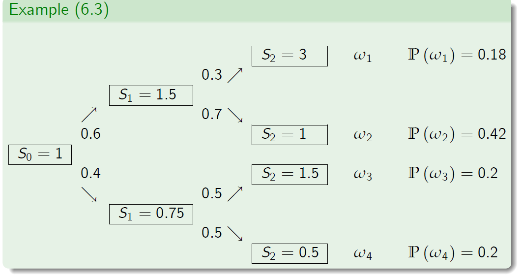
• We consider the market model in Example 6.1 once again.
• The two-period market model is composed of the following single-period market models:
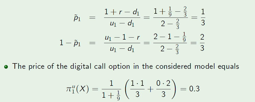
  1. \(S_1 = 1.5, S_2 = 3 and S_2 = 1\).
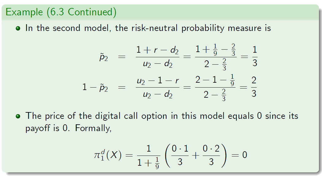
  2. \(S_1 = 0.75, S_2 = 1.5 and S_2 = 0.5\).
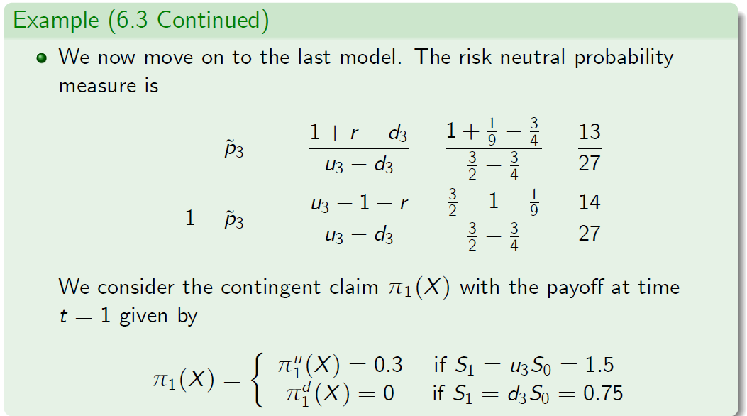
  3. \(S_0 = 1, S_1 = 1.5 and S_1 = 0.75\).
• Note that these models are elementary market models.
• Hence the unique risk-neutral probability measures can be computed using the formula

Example: Backward Induction
Example (6.3 Continued)

• Recall that if the elementary market model is arbitrage-free then it is also complete and all contingent claims can be priced using the risk-neutral probability.
• In the first model, the risk neutral probability measure is

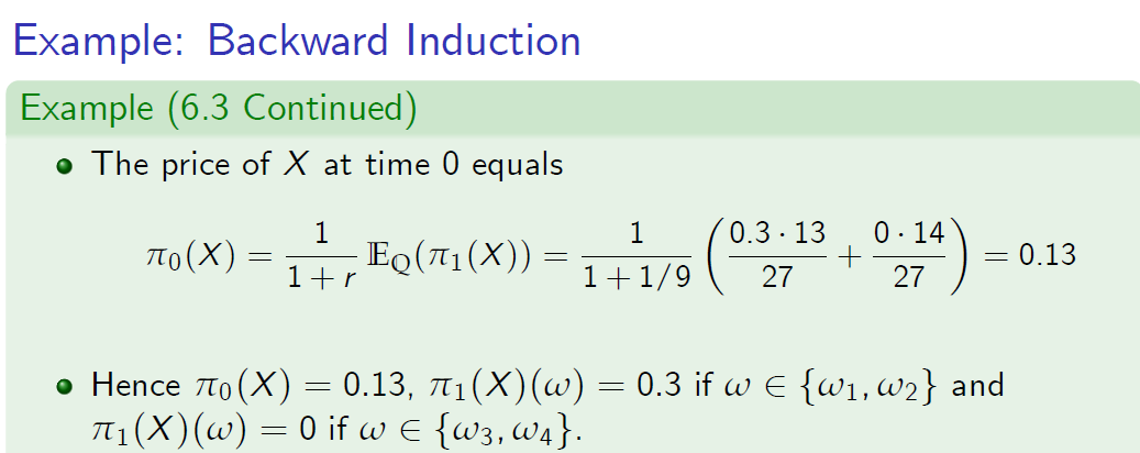
• Note that the unique risk-neutral probability measure Q in two-period market model can be recomputed as follows:

6 Completeness of Multi-Period Market Models

Completeness

As a handy criterion for the market completeness, we have the theorem,which extends the known result for the single-period case.
Theorem (6.1)
Assume that a multi-period market model \(\cal M= (B, S^1, . . . , S^n)\) is arbitrage-free. Then \(\cal\) M is complete if and only if there is only one risk-neutral probability measure, that is, \(\mathbb M = \{\hat P\}\) is a singleton.

In the context of a model decomposition, the following statements are known to hold:

• If all single-period models which compose a multi-period model are arbitrage-free then the multi-period model is also arbitrage-free.
• If they are also complete then the multi-period model is also complete.
• The converse of the above statement is also correct.

Summary of Pricing and Hedging Approaches

We examined three pricing and hedging approaches:

1. The method based on the idea of replication of a contingent claim. It can only be applied to attainable contingent claim in a complete or incomplete model and it yields the hedging strategy and arbitrage price process.
2. The method relying on the concept of a risk-neutral probability, which can be applied in either a complete or incomplete model. It furnishes the unique arbitrage price process for any attainable claim and a possible arbitrage price process for a non-attainable contingent claim. In the latter case, the price process depends on the choice of a risk-neutral probability.
3. The backward induction approach in which a multi-period market model is decomposed into a family of single-period models. Pricing is performed in a recursive way starting from the date T 􀀀 1 and moving step-by-step towards the initial date 0. Hedging strategy can also be computed provided that the claim is attainable.