Unit 6 Binomial Asset Pricing Model

Uploaded by eva

Outline

We will examine the following issues:
1 The Cox-Ross-Rubinstein Market Model
2 The CRR Call Option Pricing Formula
3 Call and Put Options of American Style
4 Dynamic Programming Approach to American Claims
美国索赔的动态规划方法
5 Examples: American Call and Put Options

Introduction

• The Cox-Ross-Rubinstein market model (CRR model) is an example of a multi-period market model of the stock price.
  二项期权定价模型（CRR模型）是股票价格多期市场模型的一个例子。
• At each point in time, the stock price is assumed to either go ‘up’ by a fixed factor u or go ‘down’ by a fixed factor d.
  在每一个时间点，股票价格都被假定为以固定因子u“上升”或以固定因子d“下降”。
• Only three parameters are needed to specify the binomial asset pricing model: u > d > 0 and r > -1.
  二项资产定价模型只需要三个参数：u>d>0 和 r>-1。

• Note that we do not postulate that d < 1 < u.
  注意，我们没有假设 d < 1 < u

• The real-world probability of an ‘up’ movement is assumed to be the same 0 < p < 1 for each period and is assumed to be independent of all previous stock price movements.
  假设每个时期的实际“上涨”概率为 0< p <1， 并且与之前的所有股价变动无关。

Bernoulli Processes

Definition (Bernoulli Process)

定义（伯努利过程)

A process
\(X= (X_t)_{0 \leq t \leq T}\)

on a probability space \((\Omega,\cal F,\mathbb P)\) is called a Bernoulli process with parameter 0 < p < 1 if the random variables \(X_1, X_2 ,…,X_T\)are independent and have the following common probability distribution
概率空间\((\Omega,\cal F,\mathbb P)\)上的过程\(X = (X_t)_{\leq t \leq T}\)称为参数为0< P <1 的 伯努利过程，如果随机变量 \(X_1,X_2, . . . ,X_T\) 是独立的，具有以下公共概率分布

\[\mathbb p (X_t = 1) = 1 - \mathbb P(X_t = 0) = p.\]

Definition (Bernoulli Counting Process)

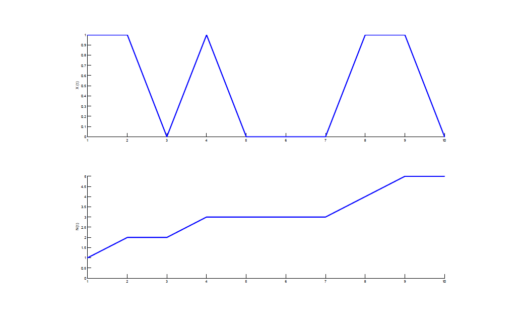
The Bernoulli counting process \(N = (N_t )_{\leq t \leq T} \) is defined by setting \(N_0 = 0\) and, for every t = 1, . . . ,T and \(\omega \in \Omega \),

伯努利计数过程 \(N_t (\omega) := X_1(\omega) + X_2(\omega) + ... + X_t (\omega).\)

The process N is a special case of an additive random walk.
过程 N 是可加性随机游走的特例。

Stock Price

Definition (Stock Price)

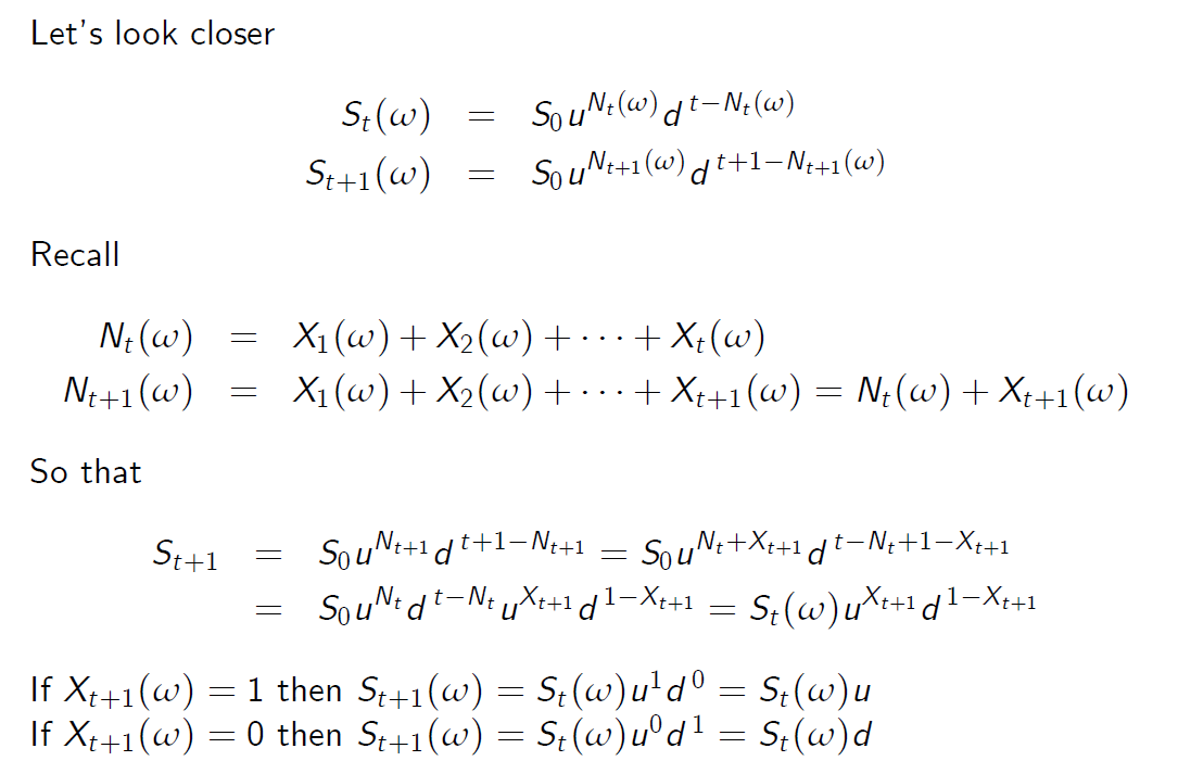
The stock price process in the CRR model is defined via an initial value \(S_0 > 0\) and, for \(1 \leq t \leq T\) and all \(\omega \in \Omega\),
CRR模型中的股票价格过程是通过初始价值\(S_0 > 0\)和对于\(1 \leq t \leq T\)和所有的\(\omega \in \Omega\)

\[S_t (\omega) := S_0 u^N_t (\omega)d^t-N_t (\omega).\]

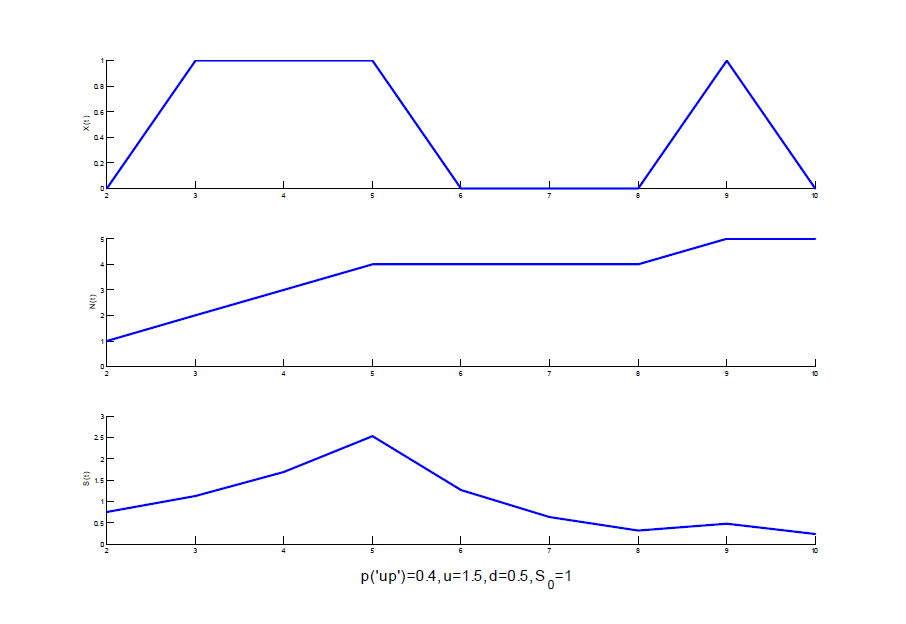
• The underlying Bernoulli process X governs the ‘up’ and ‘down’ movements of the stock. The stock price moves up at time t if \(X_t (\omega) = 1\) and moves down if \(X_t (\omega) = 0\).

基本的伯努利过程X控制着股票的“上升”和“下降”运动。如果 \(X_t (\omega) = 1\)，股票价格在时间t上升，如果\(X_t (\omega) = 0\)，股票价格下降。

• The dynamics of the stock price can be seen as an example of a multiplicative random walk.
  股票价格的动态可以看作是乘性随机游走的一个例子。

• The Bernoulli counting process N counts the up movements. Before and including time t, the stock price moves up \(N_t\) times and down \(t - N_t \) times.

伯努利计数过程N计算上升运动。在时间t之前（包括时间t），股票价格向上移动\(N_t\)次，向下移动\(t - N_t \)次。

Distribution of the Stock Price

• For each t = 1, 2, . . . ,T, the random variable \(N_t\) follows a binomial distribution with parameters p and t.
  对于每个t=1，2, … ,T，随机变量\(N_t\)遵循参数p和T的二项分布。

• Specifically, for every t = 1, . . . ,T and k = 0, . . . , t we have that
  具体来说,

• Hence the probability distribution of the stock price \(S_t\) at time t is given by
  因此，时间t时股票价格的概率分布\(S_t\)由下式给出

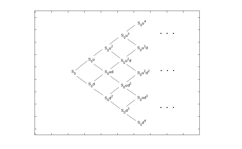
Stock Price Lattice

股票价格结构

Risk-Neutral Probability Measure

风险中性概率测度

Proposition (7.1)

Assume that d < 1 + r < u. Then a probability measure \(\mathbb {\widetilde P}\) on \((\Omega,\cal F_T )\) is a risk-neutral probability measure for the CRR model \(\cal M= (B, S)\) with parameters p, u, d, r and time horizon T if and only if:
假设 d < 1+r < u ，那么，\((\Omega,\cal F_T )\)上的概率测度\(\mathbb {\widetilde P}\)是具有参数 P，u，d，r 和时间范围T的CRR模型\(\cal M= (B, S)\)的风险中性概率测度，当且仅当：

1. \(X_1,X_2,X_3, . . . ,X_T\) are independent under the probability measure \(\mathbb {\widetilde P}\),
   \(X_1,X_2,X_3, . . . ,X_T\)在概率测度\(\mathbb {\widetilde P}\)下是独立的

2. 0 < ˜p := \( \mathbb {\widetilde P} (X_t = 1) < 1\) for all t = 1, . . . ,T,
3. ˜pu + (1 - ˜p)d = (1 + r ), where X is the Bernoulli process governing the stock price S. 其中X是控制股价S的伯努利过程。

Proposition (7.2)

If d < 1 + r < u then the CRR market model M= (B, S) is arbitrage-free and complete.
如果 d < 1 + r < u 则 CRR市场模型M= (B, S) 是完全无套利的。

Since the CRR model is complete, the unique arbitrage free price of any European contingent claim can be computed using the risk-neutral valuation formula
由于CRR模型是完整的，因此可以使用风险中性估值公式计算任何欧洲未定权益的唯一无套利价格。

我们将把这个公式应用于股票的欧式看涨期权。

2 The CRR Call Option Pricing Formula

CRR Call Option Pricing Formula

CRR看涨期权定价公式

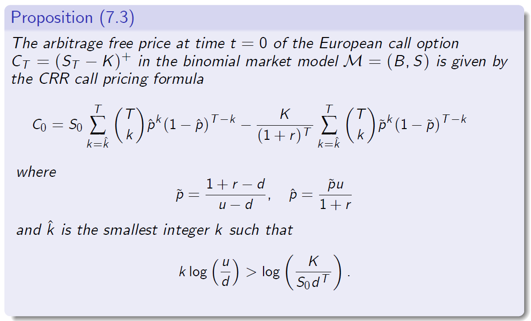
在二项市场模型M=（B，S）中，欧式看涨期权 \(C_T\) 在 t=0 时的无套利价格由 CRR 看涨定价公式给出

ˆk是最小整数k，使得

Proof of Proposition 7.3

命题证明7.3

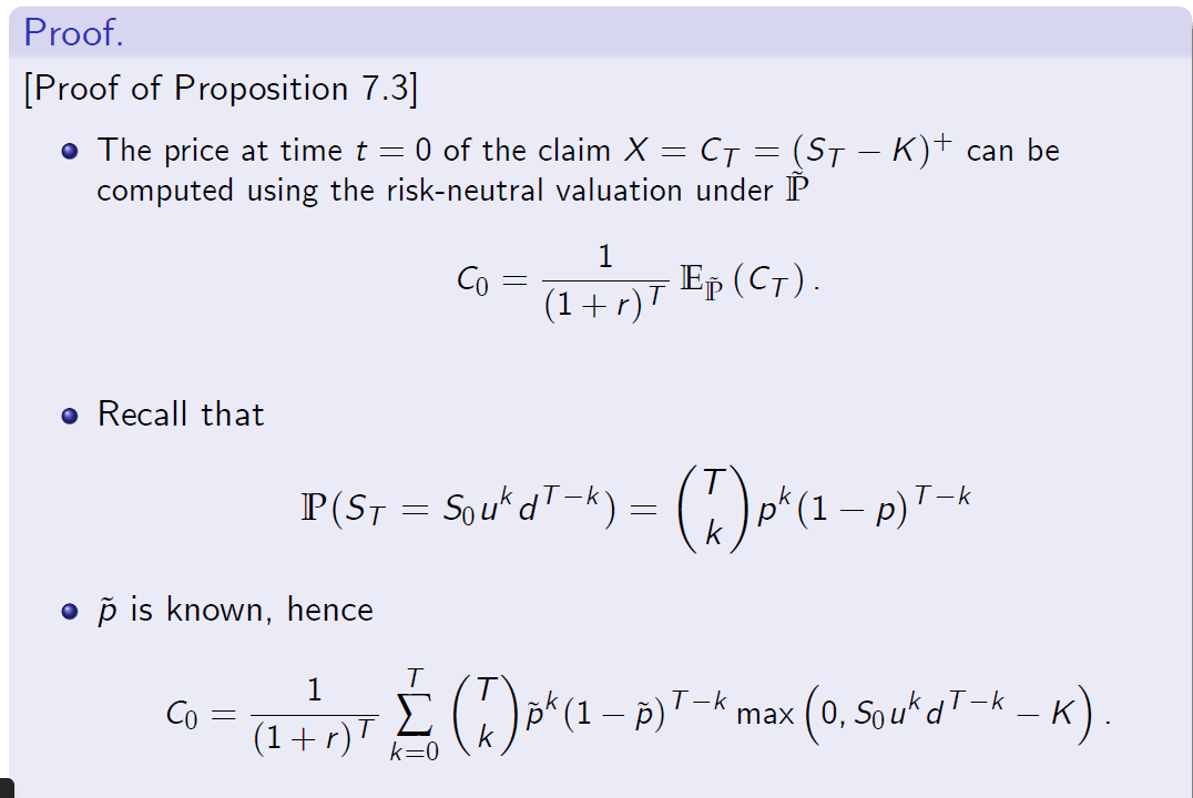
债权X的价格在t=0时可以使用概率测度P下的风险中性估值进行计算

[Proof of Proposition 7.3]

• Recall we are interested in \((S_0 u^k d^{T-k} - K)^+\)

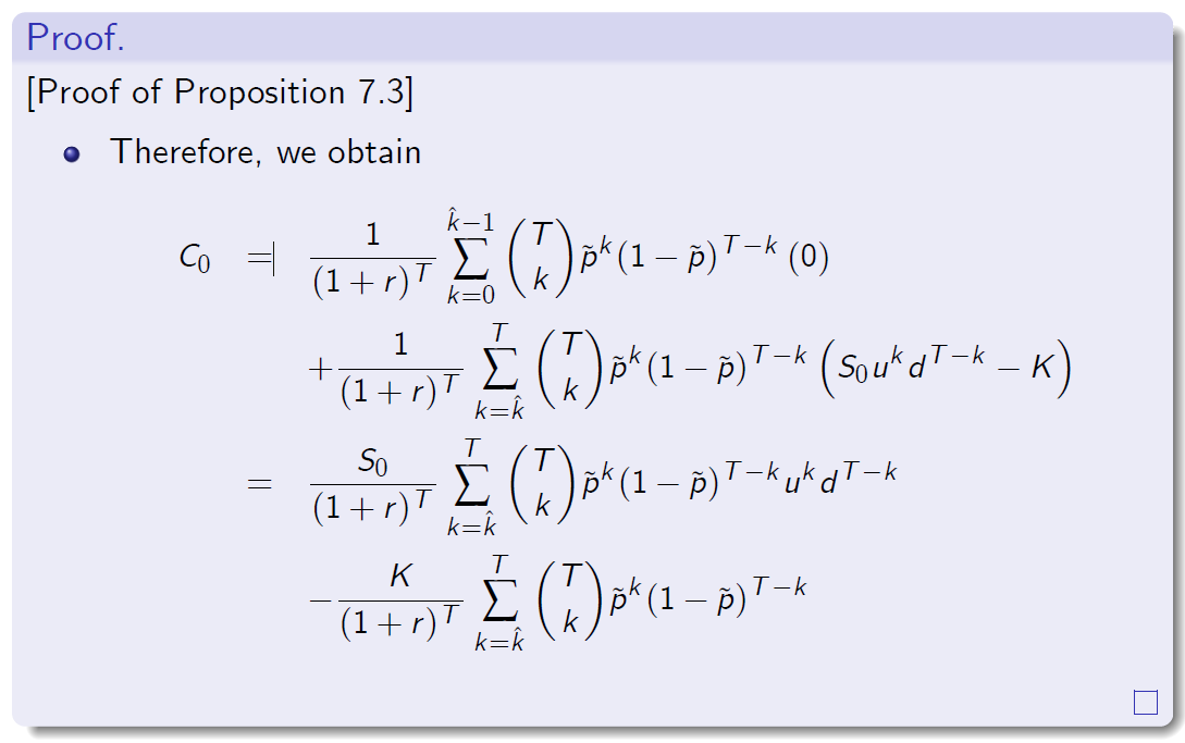
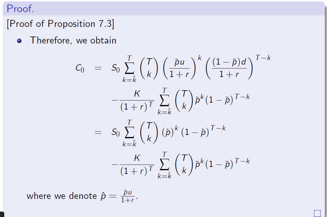
• Define \(\hat k\) to be the smallest non-negative integer k such that \(S_0 u^k d^{T-k} > K\). If \(\hat k > T\) then \(S_0 u^k d^{T-k} \leq K \) and \(C_0 = 0\).
  定义\(\hat k\)为最小的非负整数k

• Otherwise we have a chance to get some money.
  否则我们就有机会得到一些钱。
• Note

so this is just a way to write condition for the first occurence of \(S_0 u^k d^{T-k}- K > 0\).
所以这只是为\(S_0 u^k d^{T-k}- K > 0\)的第一次出现写条件的一种方法。

• We define \(\hat k = \hat k (S_0,T)\) as the smallest integer k such that the last inequality is satisied. If there are less than \(\hat k\) upward movements the option will expire worthless.
  我们定义\(\hat k = \hat k (S_0,T)\)为最小整数 k，使最后一个不等式满足。如果有少于 \(\hat k\) 的向上移动，期权将失效。

Put-Call Parity

买卖权平价关系

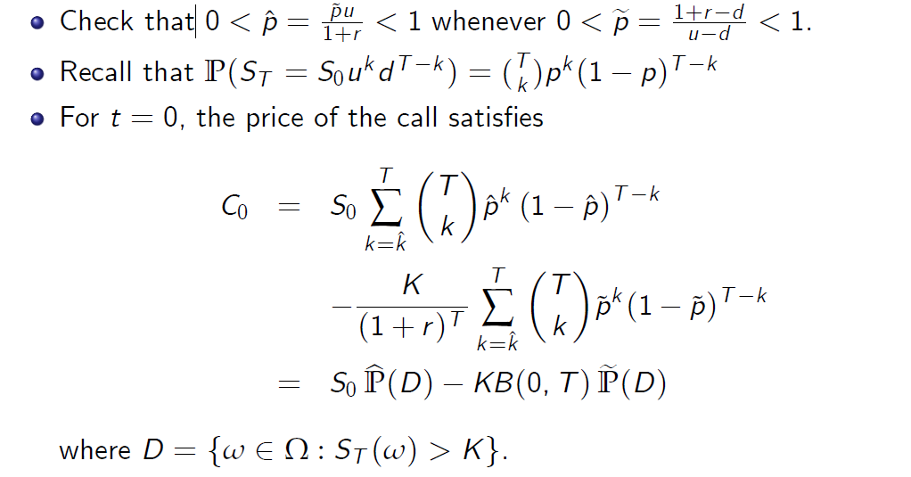
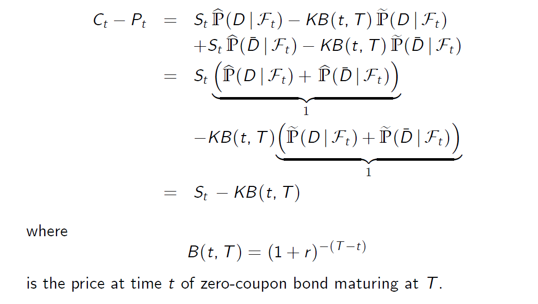
We started with t = 0, but the same analysis is true for any t. It is easy to demonstrate that

我们从t=0开始，但是同样的分析对任何t都适用。很容易证明这一点

Similarly, for a put option

Therefore, put-call parity holds at any date t = 0, 1, . . . ,T

3 Call and Put Options of American Style

American Options

• In contrast to a contingent claim of European style, a claim of American style can by exercised by its holder at any date before its expiration date T.
  与欧式未定权益不同，美式未定权益的持有人可以在其到期日T之前的任何日期行使。

Definition (American Call and Put Options)
定义（美式看涨期权和看跌期权） An American call (put) option is a contract which gives the holder the right to buy (sell) an asset at any time \(t \leq T\) of her/his choice at strike price K.
美式看涨期权（看跌期权）是一种合约，它赋予持有人在任何时候\(t \leq T\)以行使价格K购买（出售）自己选择的资产的权利。

• In the study of American options, we are concerned with the price process and the’optimal’ exercise policy by its holder.
  在美式期权的研究中，我们关注的是美式期权的价格过程及其持有者的“最优”行使策略。
• If the holder of an American option exercises it at \(\cal t \in \) [0,T], t is called the exercise time.
  如果美式期权持有人在\(\cal t \in \) [0，t]行使期权，t称为行使时间。

American Call Option

美式看涨期权

Definition

By an arbitrage free price of the American call we mean a price process \(C_t^a\) , \(t \leq T\), such that the extended financial market model - that is, a market with trading in riskless bonds, stocks and the American call option
美式看涨期权的无套利价格指的是一个价格过程\(C_t^a\)，\(t \leq T\)，即扩展的金融市场模型，即一个交易无风险债券、股票和美式看涨期权的市场 -remains arbitrage-free.
保持无套利 By definition, the arbitrage free price of American call option
根据定义，美式看涨期权的无套利价格

Proposition (7.4)

The price of an American call option in the CRR arbitrage-free market model with \(r \geq 0\) coincides with the arbitrage price of a European call option with the same expiry date and strike price.
在具有\(r \geq 0\)的CRR无套利市场模型中，美式看涨期权的价格与具有相同到期日和执行价格的欧式看涨期权的套利价格一致。

Proof of Proposition 7.4
Proof.
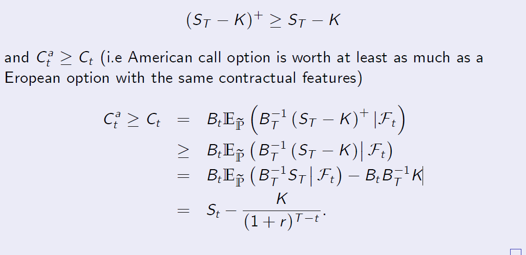
[Proof of Proposition 7.4] For simplicity, we assume r > 0. Obviously
为了简单起见，我们假设r>0。很明显

• The result only holds for non-dividend-paying stock.
  这个结果只适用于不派息的股票。

• The proof requires r > 0. It means that the similar proof for a put option might require r < 0, which is not realisic. In fact, we see a number of examples further in the course when it is optimal to exercise put option early.
  证明要求r>0。这意味着对于看跌期权的类似证明可能需要r<0，这是不现实的。事实上，在本课程中，我们还看到了许多例子，说明尽早行使看跌期权是最佳的。

American Put Option

美式看跌期权

• Recall that the American put is an option to sell a specified number of shares, which may be exercised at any time before or at the expiry date T.
  回想一下，美式看跌期权是一种出售特定数量股票的期权，可以在到期日T之前或到期日T的任何时间行使。

By definition, the arbitrage free price Pat of an American put option equals
根据定义，美式看跌期权的无套利价格等于

4 Dynamic Programming Approach to American Claims

Dynamic Programming Recursion

动态规划递归

• The stopping time \(\cal t_t^\) is called the rational exercise time of an American put option that is assumed to be still alive at time t.
  停止时间\(\cal t_t^\)被称为美式看跌期权的合理行使时间，该期权假定在时间t仍然有效。

• By an application of the classic Bellman principle (1952), one reduces the optimal stopping problem in Proposition 7.5 to an explicit recursive procedure for the value process.
  通过应用经典的贝尔曼原理（1952），我们将命题7.5中的最优停止问题简化为值过程的显式递归过程。
• We now show how to arrive to the dynamic programming recursion for the value of an American put option. The American call option can be treated similarly.
  我们现在展示如何得到美式看跌期权价值的动态规划递归。美式看涨期权也可作类似处理。
• Note that this is an extension of the backward induction approach to the valuation of European contingent claims.
  请注意，这是向后归纳法对欧洲或有债权估值的扩展。

Dynamic Programming Recursion Corollary (Bellman Principle)
推论（贝尔曼原理）

Let the non-negative adapted process U be deined recursively by setting
让非负适应过程 U 可以通过设置

Then the arbitrage free price \(P_t^a\) of the American put option at time t equals \(U_t\) and the rational exercise time after time t admits the following representation
那么，美式看跌期权在t时刻的无套利价格\(P_t^a\)等于\(U_t\)，并且t时刻之后的合理行使时间允许如下表示

Dynamic Programming Recursion

• It is also possible to show directly that the price \(P_t^a\) satises the recursive relationship, for \(t \leq T - 1\),
  对于\(t \leq T - 1\)），也可以直接表明价格\(P_t^a\)满足递归关系，

subject to the terminal condition \(P_T^a = (K - S_T )^+\).根据终端条件

• In the case of the CRR model, this formula reduces the valuation problem to the simple single-period case.
  在CRR模型的情况下，这个公式将估值问题简化为简单的单期情况。
• To show this we shall argue by contradiction. Assume first that (1) fails to hold for t = T - 1. If this is the case, one may easily construct at time T - 1 a portfolio which produces riskless profit at time T. Hence, we conclude that necessarily
  为了表明这一点，我们将用矛盾来辩论。首先假设（1）不能保持 t=t-1 。如果是这样的话，我们可以很容易地在时间 T-1 构建一个在时间 T 产生无风险利润的投资组合

• This procedure may be repeated as many times as needed.
  此程序可根据需要重复多次。

American Put Option: Summary

美式看跌期权：总结

To summarize:

• In the CRR model, the arbitrage pricing of the American put option reduces to the following recursive recipe, for \(t \leq T - 1\),
  总结一下：

-在CRR模型中，美式看跌期权的套利定价简化为如下递归公式，即\(t \leq T - 1\)，

The quantities \(P_{t+1}^{au}\) and \(P_{t+1}^{ad}\) represent the values of the American put in the next step corresponding to the upward and downward movements of the stock price starting from a given node on the CRR lattice.
数量\(P_{t+1}^{au}\) and \(P_{t+1}^{ad}\)表示美国人在下一步中投入的价值，对应于股票价格从CRR晶格上的给定节点开始的上下波动。

American Call Option: Summary

美式看涨期权：总结

To summarize:
总结一下：

In the CRR model, the arbitrage pricing of the American call option reduces to the following recursive recipe, for \(t \leq T - 1\),
在CRR模型中，美式看涨期权的套利定价简化为如下递归公式，即

The quantities \(P_{t+1}^{au}\) and \(P_{t+1}^{ad}\) represent the values of the American call in the next step corresponding to the upward and downward movements of the stock price starting from a given node on the CRR lattice.
数量\(P_{t+1}^{au}\) and \(P_{t+1}^{ad}\)表示下一步美式看涨期权的价值，对应于股票价格从CRR晶格上的给定节点开始的向上和向下运动。

5 Examples: American Call and Put Options

Example: American Call Option

Example (7.1)

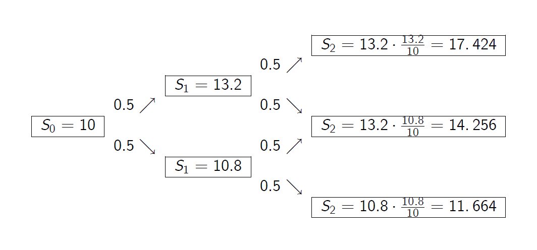
• We consider here the CRR binomial model with the horizon date T = 2 and the risk-free rate r = 0.2.
  我们在这里考虑CRR二项式模型，其水平日期T=2，无风险利率r=0.2。
• The stock price S for t = 0 and t = 1 equals
  t=0和t=1的股票价格S等于 \(S_0 = 10, S_1^u=13.2, S_1^d= 10.8.\) Let \(X^a\) be the American call option with maturity date T = 2 and the following payoff process
  设\(X^a\)为美式看涨期权，到期日T=2，支付过程如下

\(g(S_t , t) = (S_t - K_t )^+.\)
The strike \(K_t\) is variable and satisfies
\(K_0 = 9, K_1 = 9.9, K_2 = 12.\)

Example: American Call Option

例如：美式看涨期权

Example (7.1 Continued)

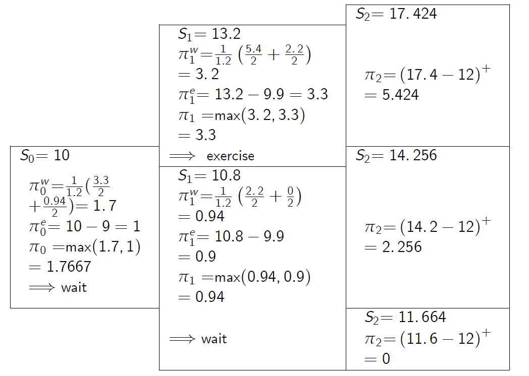
• We will first compute the arbitrage price \(\pi_t (X^a)\) of this option at times t = 0, 1, 2 and the rational exercise time \(t_0^* \).
  我们将首先计算t=0，1，2和合理行使时间\(t_0^* \)时该期权的套利价格\(\pi_t (X^a)\)。
• Subsequently, we will compute the replicating strategy for \(X^a\) up to the rational exercise time \(t_0^{}\).
  随后，我们将计算Xa到合理运动时间 \(t_0^\) 的复制策略.

• The second exhibit represents the price of the call option.

Example: Replicating Strategy

复制策略

Example (7.1 Continued)

• Holder. The rational holder should exercise the American option at time t = 1 if the stock price rises during the first period. Otherwise, the option should be held till time 2. Hence \(t_0^* : \Omega \to \{0, 1, 2\} \) equals
  如果股票价格在第一阶段上涨，理性持有人应该在t=1时行使美式期权。否则，该选项应保留到时间2。

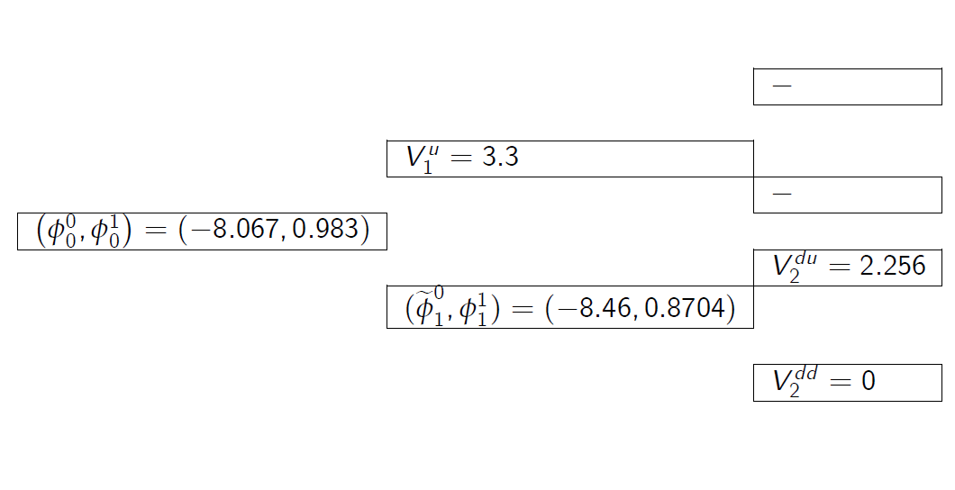
• Issuer. We now take the position of the issuer of the option. At t = 0, we need to solve

Example: Replicating Strategy Example (7.1 Continued)

• If the stock price rises during the first period, the option is exercised and thus we do not need to compute the strategy at time \(t_0^* : \Omega \to \{0, 1, 2\} \).
  如果股票价格在第一阶段上涨，期权被行使，因此我们不需要计算时间\(t_0^* : \Omega \to \{0, 1, 2\} \)的策略。
• If the stock price falls during the first period, we solve
  如果股票价格在第一阶段下跌，我们解决

• Note that \(\widetilde \phi ^0_1 = 8.46 \) is the amount of cash borrowed at time 1, rather than the number of units of the savings account B.
  注意，\(\widetilde \phi ^0_1 = 8.46 \)是在时间1借入的现金金额，而不是储蓄账户的单位数。
• The replicating strategy \(\phi = (\phi^0, \phi^1)\)is defined at time 0 for all w and it is defined at time 1 on the event \({\omega_3,\omega_4}\) only.
  复制策略\(\phi = (\phi^0, \phi^1)\)在时间0为所有w定义，并且仅在事件\({\omega_3,\omega_4}\)的时间 1 定义。

Example: American Call Option vs. European Call Option

示例：美式看涨期权与欧式看涨期权

Example (7.1)

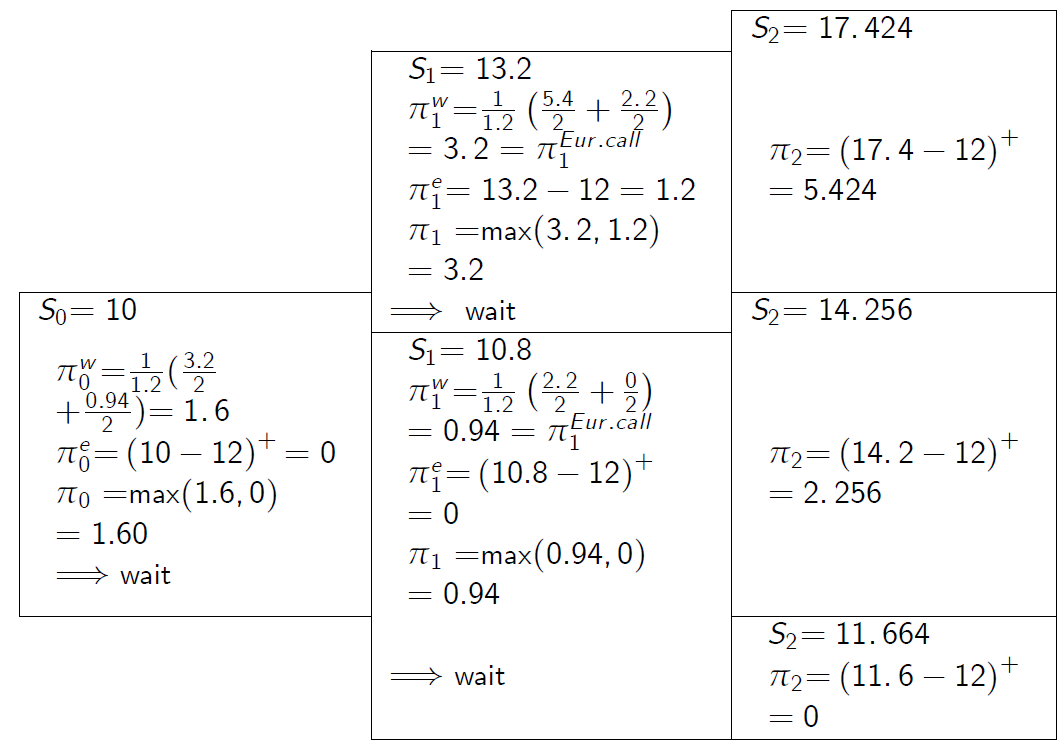
• Consider the same setup but \(K_t = 12\) and does not depend on time.
  考虑相同的设置，但是\(K_t = 12\)，并且不依赖于时间。

欧洲看涨期权的执行价相同。 The same strike price is for the European Call option.

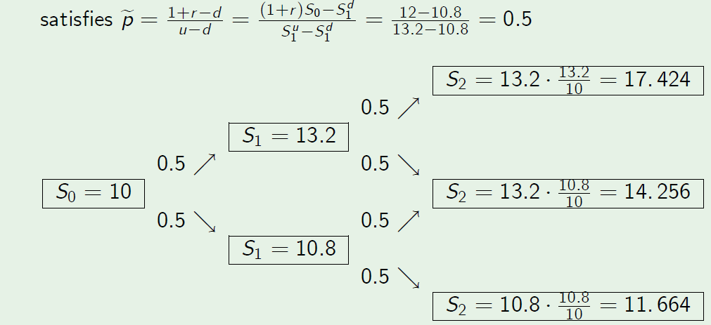
• We start by noting that the unique risk-neutral probability measure \(\mathbb P\) satisfies
  我们首先注意到唯一的风险中性概率测度\(\mathbb P\)满足

Derivation of u and d from r and \(\sigma\)

从r和s推导u和d

• the parameters r and \(S_0\) can be observed in real financial markets, but the parameters u and d are only a model idealization and can not be directly determined by observation of real world data people trading on stock markets study a different parameter, which they call volatility and which reects a property of the corresponding continuous time model, also known as the Black-Scholes model
  参数r和\(S_0\)可以在真实的金融市场中观察到，但参数u和d只是模型的理想化，不能通过观察真实世界的数据来直接确定在股票市场上交易的人们研究不同的参数，他们称之为波动率，它反映了相应的连续时间模型的一个特性，也被称为布莱克-斯科尔斯模型

• From the market data for stock prices, one can estimate the stock price volatility s per one time unit (typically, one year).
  根据股票价格的市场数据，我们可以估计每一时间单位（通常是一年）的股票价格波动率。
• Note that until now we assumed that t = 0, 1, 2, . . . ,T, which means that \(\Delta t = 1\). In general, the length of each period can be any positive number smaller than 1. We set \(n = T/\Delta t\).
  注意到现在我们假设t=0，1，2。，T，这意味着\(\Delta t = 1\)。一般来说，每个周期的长度可以是任何小于1的正数。我们设置\(n = T/\Delta t\)。

Derivation of u and d from r and \(\sigma\)

Two widely used conventions for obtaining u and d from \(\sigma\) and r are:

• The Cox-Ross-Rubinstein (CRR) parametrisation:

• The Jarrow-Rudd (JR) parameterisation:

The CRR parameterisation

Proposition (7.5)

Assume that \(B_{k \Delta t} = (1 + r\Delta t)^k \)for every k = 0, 1, . . . , n and

provided that \(\Delta_t\) is sufficiently small.

Proof.

[Proof of Proposition 7.5] The risk-neutral probability measure for the CRR model is given by

The CRR parameterisation Proof. [Proof of Proposition 7.5] Under the CRR parametrisation, we obtain

The Taylor expansions up to the second order term are

The CRR parameterisation Proof. [Proof of Proposition 7.5] By substituting the Taylor expansions into the risk-neutral probability measure, we obtain

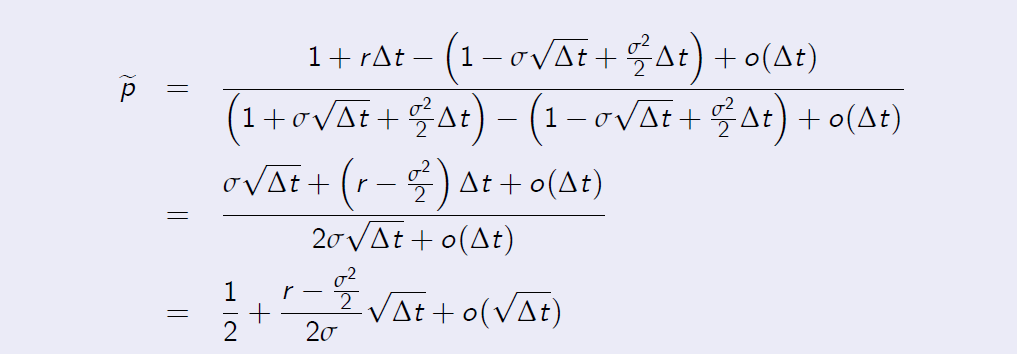
as was required to show.

The CRR parameterisation

• To summarise, for \(\Delta_t\) sufficiently small, we get

• Note that \(1 + r \Delta t \approx e^{r \Delta t} \)when Dt is sucffiently small.

• Hence the risk-neutral probability measure can also be represented as follows
  

• More formally, we can define \(\hat r\) such that \((1+ \hat r )n = e^{rT}\) for a fixed T and \(n = T/\Delta t\) then \(\hat r \approx r\Delta t\) since \(ln(1 + \hat r ) = r \Delta t\) and \(ln(1 + \hat r ) \approx \hat r\) when \(\hat r\) is close to zero.

The Binomial Asset Pricing Model

• in applications one generally chooses a small time unit
  

• though simple by its construction, the binomial market model is a very powerful tool in practical applications, if one chooses \(\Delta t\) very small, in fact one then obtains a reasonably good approximation of trading in continuous time
• the CRR options pricing formula then approximates the Black-Scholes options pricing formula (see Black and Scholes (1973) and later in this module). In fact, the Black-Scholes options pricing formula can be derived by letting the time increments in the CRR options pricing formula go to zero.

The Binomial Asset Pricing Model
To implement a numerical algorithm for the evaluation of options and contingent claims we introduce the notation

The numerical values \(S_{ji}\) represent the price of the stock at time i , when counting from initial time 0 and the stock has gone up j times.

• let X be a contingent claim. We can compute an arbitrage free price for X at time \(i \Delta t\) via the formula

• by Definition of the conditional expectation this random variable is \(\cal F_i\)-measurable, meaning that it depends on information gathered up to time \(i \Delta t\)

The Binomial Asset Pricing Model

• If X is of the type \(h(S_M)\), meaning that the payo¤ only depends on the terminal value of the stock, then one can use the independence of the \(\frac {Si} {S_{i-1}}\) ‘s and show that \(V_i\) depends on this information only through the price of the stock Si at time \(i \Delta t\).
• The latter re‡ects the Markov property of the stock price process in the binomial model. We will later see this property occurring in more complicated models.

We are now able to write the random variable Vi as a function of Si . We then denote \(V_{i}\) := price of X at time i if stock price is \(S_{i}\)

The Binomial Asset Pricing Model At terminal time T ( i = M ) the contingent claim pays off:
\(V_{jM}=h(S_{jM})\)

for all j = 0, …,M. We use this as the initialization of our scheme and work backward in time.

• using the tower property of the conditional expectation, one derives that

and therefore one obtains the backward step
This is so-called Bellman equation.

• using our initialization we now iterate the backward step in order to compute \(V_00\), the price of the contingent claim at present time 0

Binomial Asset Pricing Model: Matlab

function [price, lattice] = LatticeEurCall(S0,K,r,T,sigma,N)
deltaT = T/N;
u=exp(sigma * sqrt(deltaT));
d=1/u;
p=(exp(rdeltaT) - d)/(u-d);
lattice = zeros(N+1,N+1);
for i=0:N
lattice(i+1,N+1)=max(0 , S0(u^i)(d^(N-i)) - K);
end
for j=N-1:-1:0
for i=0:j
lattice(i+1,j+1) = exp(-rdeltaT) * …
(p * lattice(i+2,j+2) + (1-p) * lattice(i+1,j+2));
end
end
price = lattice(1,1);

Example: American Put Option

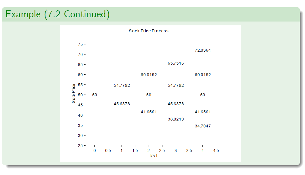
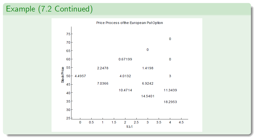
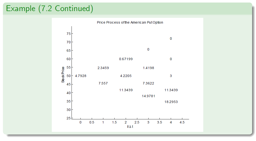
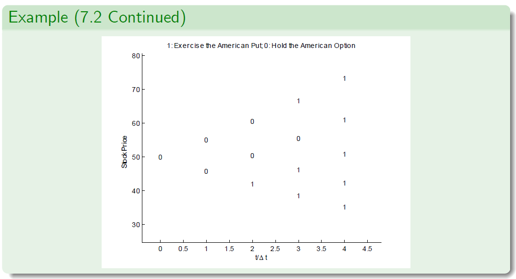
Example (7.2 - CRR Parameterisation)

• Let the annualized variance of logarithmic returns be \(\sigma^2 = 0.1\).
• The interest rate is set to r = 0.1 per annum.
• Suppose that the current stock price is \(S_0 = 50\).
• We examine European and American put options with strike price K = 53 and maturity T = 4 months (i.e. \(T = \frac{1}{3}\)).
• The length of each period is \(\Delta t = \frac{1}{12}\) , that is, one month.
• Hence \(n = \frac{T} {\Delta t}\) = 4 steps.
• We adopt the CRR parameterisation to derive the stock price.
• Then u = 1.0956 and d = 1/u = 0.9128.
• We compute \(1 + r\Delta t = 1.00833 \approx e^{r\Delta t}\) and \(\widetilde p = 0.5228\).

The JR parameterisation

The next result deals with the Jarrow-Rudd parametrisation.

Proposition (7.9)

Let \(B_{k\Delta t} = (1 + r\Delta t)^k\) for k = 0, 1, . . . , n. We assume that

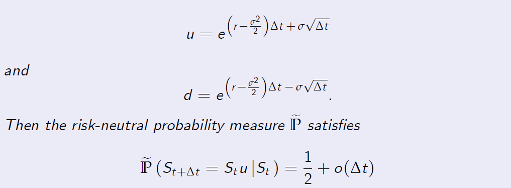
provided that Dt is sufficiently small.

The JR parameterisation

Proof.

[Proof of Proposition 7.9] Under the JR parametrisation, we have

The Taylor expansions up to the second order term are

Example: American Put Option

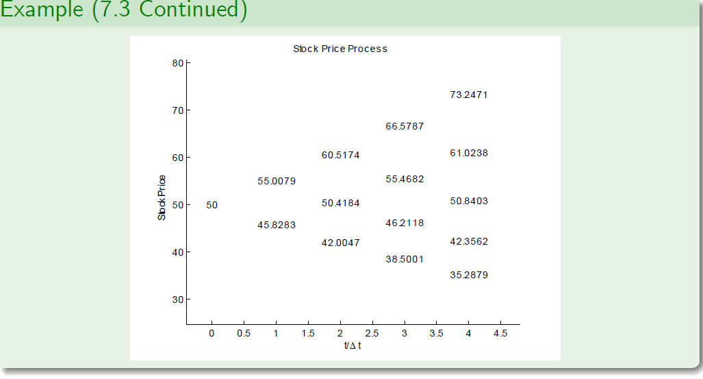
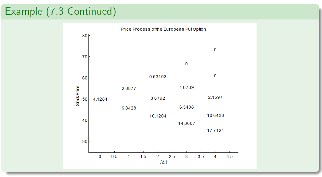
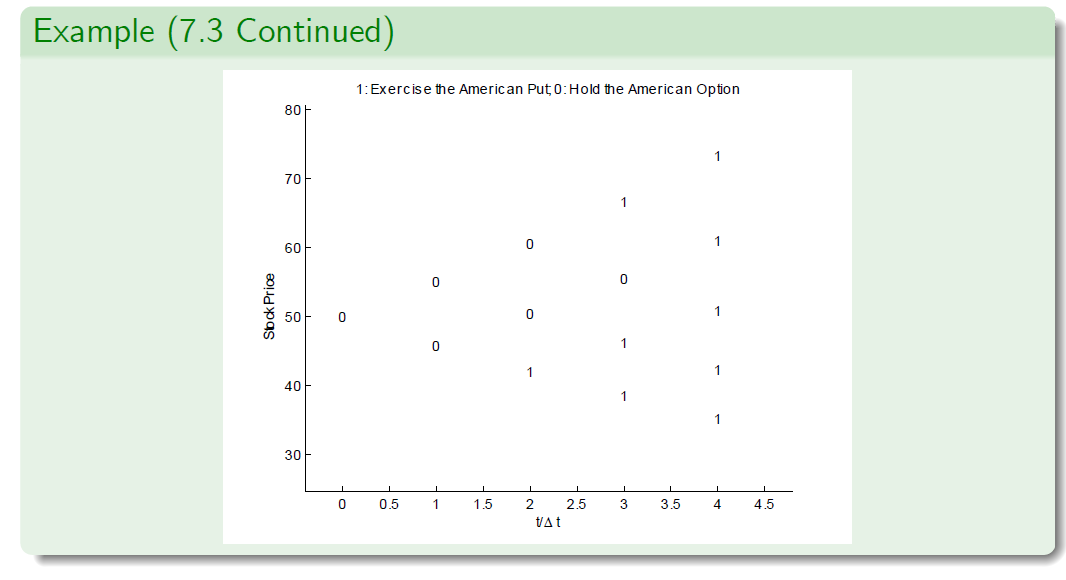
Example (7.3 -JR Parameterisation)

• We consider the same problem as in Example 7.2, but with parameters u and d computed using the JR parameterisation. We obtain u = 1.1002 and d = 0.9166.
• As before, \(1 + r\Delta t = 1.00833 \approx e^{r\Delta t}\) , but \(\widetilde p = 0.5\).
• We compute the price processes for the stock, the European put option, the American put option and we find the rational exercise time.
• When we compare with Example 7.2, we see that the results are slightly di¤erent than before, although it appears that the rational exercise policy is the same.
• The CRR and JR parameterisations are both set to approach the Black-Scholes model.
• For \(\Delta t\) sufficiently small, the prices computed under the two parametrisations will be very close to one another.

\(X= (X_t)_{0 \leq t \leq T}\)