Unit 7 The Black-Scholes Model

Uploaded by eva

Outline

We will examine the following issues:
1 Wiener Process and its Properties
2 The Black-Scholes Market Model
3 The Black-Scholes Call Option Pricing Formula
4 The Black-Scholes Partial Differential Equation

1 Wiener Process and its Properties

Wiener Process

• The Brownian motion is a mathematical model used to describe the random movements of particles. It was named after Scottish botanist Robert Brown (1773-1858).
• The Brownian motion is also known as the Wiener process in honour of American mathematician Norbert Wiener (1894-1964). The Wiener process
  is widely used to model uncertainty in engineering, economics and finance.
• It is known that almost all sample paths of the Wiener process are continuous functions of the time parameter, but they are non-differentiable everywhere.

Wiener Process: Definition

Definition (Wiener Process: Equivalent Definition)
A stochastic process \(W = (W_t , t \in \mathbb R_+)\) on \(\Omega\) is called the Wiener process if the following conditions hold:
1 W(0) = 0.
2 Sample paths of W are continuous functions.
3 For any \(0 \leq s < t, W(t) -W(s) \sim N (0, t - s)\) where \(N(μ, \sigma^2)\) denotes the normal distribution with expected value μ and variance \(\sigma^2\). 4 The process \(W_t\) has independent increments, i.e. for any \(0 \leq t_1 < t_2 < … < t_n\),
\(W(t_1),W(t_2) -W(t_1), . . . ,W(t_n) -W(t_{n-1})\) are mutually independent.

Existence of the Wiener Process

• The Brownian motion was used in Physics to describe the diffusion movements of particles (in particular, by Einstein in his famous paper published in 1905).
• The existence of a process satisfying the definition of a Wiener process is not obvious, however.
• The following theorem was first rigorously established by Norbert Wiener in the paper published in 1923.

Theorem (Wiener’s Theorem)

There exists a probability space \((\Omega,\cal F,\mathbb P)\) and a process W defined on this space, such that conditions (1)-(4) of the definition of the Wiener process are met.

Wiener Process: Sample Paths

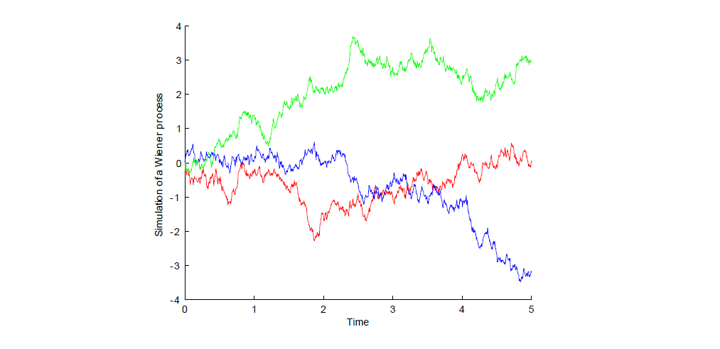
Figure: Three paths of a Wiener process with \(\Delta t = 0.005\)

Distribution of the Wiener Process

• Let \(N(μ, \sigma^2)\) denote the normal distribution with mean μ and variance \(\sigma^2\). Probability distribution function (pdf) or a normally distributed variable is

• The random variable Wt has the pdf p(x, t) given by

• Hence for any real numbers \(a \leq b\)

where N is the standard normal cumulative distribution function (cdf), that is,

Markov Property

Proposition (8.1)

The Wiener process W is a Markov process in the following sense: for every \(n \geq 1\), any sequence of times \(0 < t_1 < . . . < t_n < t\) and any collection \(x_1, . . . , x_n\) of real numbers, the following holds:

for all \(x \in \mathbb R\). Moreover,

is the transition probability density function of the Wiener process.

Martingale Property

Proposition (8.2)

Let (W,F,P) be a probability space and W be the Wiener process. Then the process W is a martingale with respect to its natural filtration \(\cal F_t = \cal F_t^W\), that is, the filtration generated by W.

Proof.

[Proof of Proposition 8.2] For all \(0 \leq s < t\), using the independence of increments of W, we obtain

We conclude that W is a martingale with respect to its natural filtration.

Stochastic differential equations

Recall that differential equation

\[x(t)=f(t,x(t))\]

can be written alternatively as

\[dx(t)=f(t,x(t)) dt\]

or approximative as

\[\Delta x(t)=f(t,x(t)) \Delta t\]

with \(\Delta x(t)= x(t+\Delta t)- x(t) \)and \(\Delta t\) a small time increment.
The increment of the function x(.) over the small time interval \(\Delta t\) is given by \(f(t,x(t)) \Delta t\) (all deterministic)

1. Now, imagine that the dynamics of x(t) is a¤ected by little random shocks \(\Delta W\) generated by the increments of Brownian motion
2. More precisely, assume that (in approximation) the increment of the state variable x(.) over the time interval \(\Delta t\) is given by

1. In differential notation we write equation (3) as

and call the latter a stochastic differential equation.

The Itô formula

Assume we have a process which is the solution of the stochastic differential equation

and that we are interested in the values or more generally in the dynamic and the stochastic properties of an expression such as \(g(t) = G(t, x(t)) with G : [0,\infty) × \mathbb R \to \mathbb R\).

1. the Itô formula provides a tool, how to compute the dynamic of the transformed process g(.) with g(t) = G(t, x(t)) in terms of the dynamic of x(.)
2. it presents in a way a generalization of the chain rule of classical calculus
3. this shows to be extremely helpful when solving stochastic differential equations and is necessary to derive pricing PDE’s for option pricing problems

Theorem (Itô formula) Suppose that x(.) solves the stochastic differential equation

and that \( G : [0,\infty) × \mathbb R \to \mathbb R\) is a function with continuous partial derivatives \(G_t,G_x\) and \(G_{xx} \). Then the stochastic process g(.) defined by g(t) = G(t, x(t)) has the following dynamics

Knowing the chain-rule of classical calculus, only the middle term \(\frac{1}{2} \sigma^2(t, x(t))G_{xx} (t, x(t))\sigma^2(t, x(t))dt\) is somehow unexpected. The reason for its occurrence is the following:

1. a second order term in dW produces a first order dt, often written as \((dW(t))^2 = dt\)
2. the Itô formula can then be derived from second order Taylor approximation, taking the above rule into account, and neglecting all dt terms which are of order strictly higher than first order.
3. there is also a multi-dimensional version of the Itô formula
4. in our applications x(t) will denote the stock price and G(t, x(t)) the price of an option

Stock Price Process

• We note that the values of the Wiener process W can be negative and thus it cannot be used to directly model the movements of the stock price.
• Following Black and Scholes (1973), we postulate that the stock price process S can be described under the risk-neutral probability measure \(\mathbb P\) by the following stochastic differential equation

with a constant initial value \(S_0 > 0\).

• The term \(\sigma S_t dW_t\) is aimed to give a reasonable description of the uncertainty in the market.

• The volatility parameter \(\sigma > 0\) is used to control the size of random fluctuations of the stock price.

• It turns out that stochastic di¤erential equation (1) can be solved explicitly yielding

The process S is called the geometric Brownian motion.

• Note that St has the lognormal distribution for every t > 0.
• It can be shown that S is a Markov process. Note, however, that S is not a process of independent increments.
• We assume that the continuously compounded interest rate r is constant. Hence the savings account equals

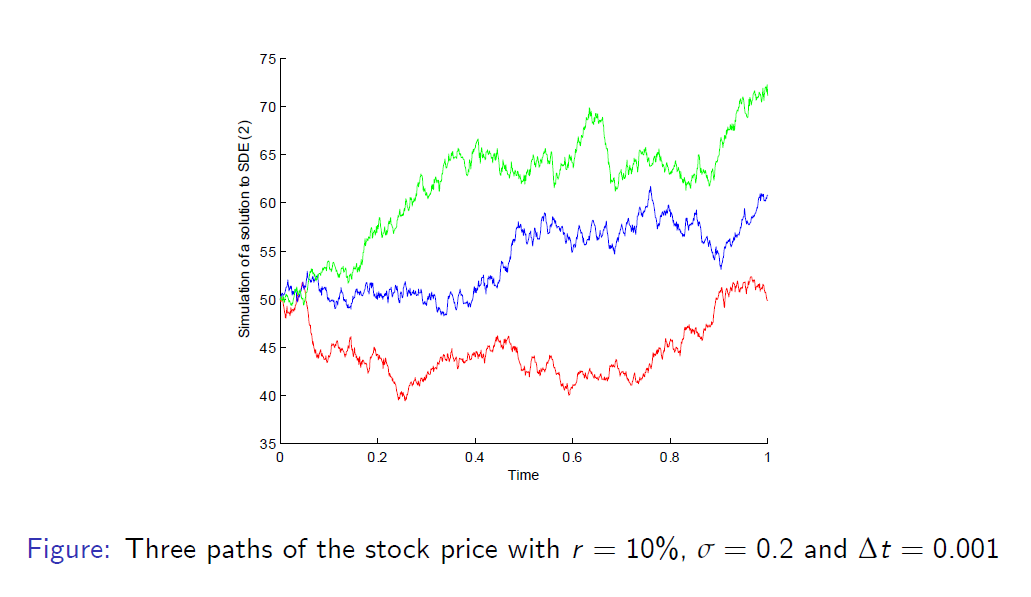
Sample Paths of Stock Price

Random Walk Approximation

• Our final goal is to examine an approximation of the Black-Scholes model by a sequence of CRR models.
• The following result is an easy consequence of the Central Limit Theorem.

Theorem (8.2)

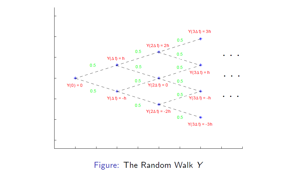
be a random walk starting at 0 with increments

and the limit exists in the sense of probability distribution.

Approximation of the Stock Price

• Recall that the JR parameterisation for the CRR binomial model postulates that

• We will show that it corresponds to a particular approximation of the stock price process S

• Suppose that \(S_s\) is known. Recall (formula (5) in this set of slides) that for all \(s \leq t\)

• Let us set \(s = t - \Delta t\) and let us replace the Wiener process \(W_t\) by the random walk \(Y_t\) in equation (5). Then we obtain

Consequently, we obtain the following approximation

We observe that this approximation of the stock price process leads to the JR parameterisation.

From discrete to continuous time

Recall Jarrow-Rudd parametrisation:

One can see the trend (drift) and (symmetric) volatility terms for the logarithm of price. Denote \(X_t = log S_t\)

In CRR model d and u could be any. We now look at particular d and u (JR parameterisation) and learn that with these d and u the log of price has clear drift and volatility components. It means that the representation has simple and intuitive form.

2 The Black-Scholes Market Model

The Black-Scholes Model \(\cal M= (B, S)\)

Assumptions of the Black-Scholes market model \(\cal M= (B, S)\):

• There are no arbitrage opportunities in the class of trading strategies.
• It is possible to borrow or lend any amount of cash at a constant interest rate \(r \geq 0\).
• The stock price dynamics are governed by a geometric Brownian motion.
• It is possible to purchase any amount of a stock and short-selling is allowed.
• The market is frictionless: there are no transaction costs (or any other costs).
• The underlying stock does not pay any dividends.

Discounted Stock Price

As in a multi-period market model, the discounted stock price \(\hat S\) is a martingale.

Proposition (8.3)

The discounted stock price, that is, the process \(\hat S\) given by the formula

is a martingale with respect to its natural filtration under \(\mathbb P\), that is, for every \(0 \leq s \leq t\),

Proof of Proposition 8.3

Proof.
[Proof of Proposition 8.3]

• We observe that equality (5) yields

• Hence if we know \(\hat S_t\) then we also know the value of \(W_t\) and vice versa. This immediately implies that \(\mathbb F^ {\hat S} = \mathbb F^W\) .

• Therefore, the following conditional expectations coincide

for any integrable random variable X

Proof.
[Proof of Proposition 8.3 (Continued)]

• We obtain the following chain of equalities

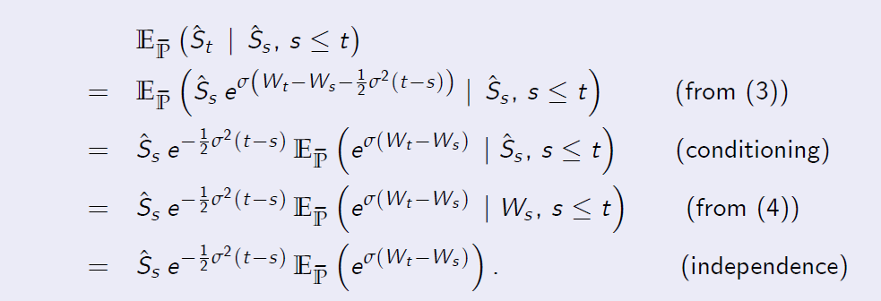
because of independence of increments.

• It remains to compute the expected value above.

Proof.
[Proof of Proposition 8.3 (Continued)]

which shows that \(\hat S\) is indeed a martingale.

Call Option

• Recall that the European call option written on the stock is a traded security, which pays at its maturity T the random amount

where \(x^+ = max (x,0)\) and K > 0 is a fixed strike.

• We take for granted that for \(t \leq T\) the price \(C_t (x)\) of the call option when \(S_t = x\) is given by the risk-neutral pricing formula

• This formula can be supported by the replication principle. This argument requires the knowledge of the It¯o stochastic integration theory with respect to the Brownian motion, as was developed by Kiyoshi It¯o (1944).

3 The Black-Scholes Call Option Pricing Formula

The Black-Scholes Call Pricing Formula

• The following call option pricing result was established in the seminal paper by Black and Scholes (1973).

Theorem (8.1)

The arbitrage price of the European call option at time \(t \leq T\) equals

and N is the standard normal cumulative distribution function.

Proof of Theorem 8.1

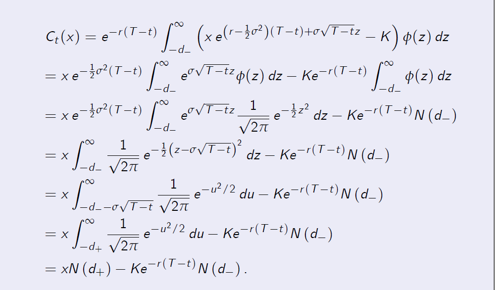
Proof. [Proof of Theorem 8.1] Our goal is to compute the conditional expectation

We can represent the stock price \(S_T\) as follows

As in the proof of Proposition 8.3, we write

where Z has the standard Gaussian probability distribution, that is, \(Z \sim N(0, 1)\).

Proof of Theorem 8.1
Proof.
[Proof of Theorem 8.1 (Continued)]

• Using the independence of increments of the Wiener process W, we obtain, for a generic value x > 0 of the stock price \(S_t\) at time t

• We denote here by f the \(\phi\) of Z, that is, the standard normal probability density function.

Proof of Theorem 8.1 Proof. [Proof of Theorem 8.1 (Continued)] It is clear that the function under the integral sign is non-zero if and only if the following inequality holds

This in turn is equivalent to the following inequality

Let us denote

Proof of Theorem 8.1 Proof. [Proof of Theorem 8.1 (Continued)]

Put-Call Parity

• The price of the put option can be computed from the put-call parity

• Specifically, the put option price equals

• It is worth noting that \(C_t > 0\) and \(P_t > 0\).
• It can also be checked that the prices of call and put options are increasing functions of the volatility parameter s (if all other quantities are fixed). Hence the options become more expensive when the underlying stock becomes more risky.
• The price of a call (put) option is an increasing (decreasing) function of r .

4 The Black-Scholes Partial Differential Equation

The Black-Scholes PDE

Proposition (8.4) Consider a path-independent contingent claim \(X = h(S_T \)), which only depends on the final price. Let the price of the contingent claim at t given the current stock price \(S_t = x\) be denoted by V (t, x). Then V (t, x) is the solution of the Black-Scholes partial differential equation

with the terminal condition V (T, x) = h(x).
Proof.
[Proof of Proposition 8.4] We will discuss this statement further in the course.

The Black-Scholes Model

A contingent claim X with the payo¤ function is h (S) can be priced by using the risk neutral probability measure \(\mathbb Q\), i.e.,

Theorem (Feynman-Kac Theorem)

Suppose function g(x) is continuous and W(t) is a Wiener process. Define

then u(t, z) solves the following partial di¤erential equation (PDE) with the boundary condition:

The Black-Scholes Model

• The Feynman-Kac theorem presented above is an elementary version.
  There are other versions.
• In the Feynman-Kac theorem, \(\mathbb P\) and W(t) can be replaced by \(\mathbb Q\) and W(t), where W(t) is a Wiener process under \(\mathbb Q\).
• The implication of the Feynman-Kac theorem is that one can price a contingent claim in the Black-Scholes model by computing expectations or solving PDEs.

The Black-Scholes Model

Proposition (5.3)

Let the price of the contingent claim at t given the current stock price \(S_t = x\) be denoted by V (t, x). Then V (t, x) is the solution of

with the boundary condition V (T, x) = h(x).

Equation (6) is called the Black-Scholes equation.

The Black-Scholes Model

Proof.

[Proof of Proposition 5.3] The price of a contingent claim with the payoff function h (S) at t given the current stock price \(S_t = x\) must satisfy

The Black-Scholes Model Proof. [Proof of Proposition 5.3]

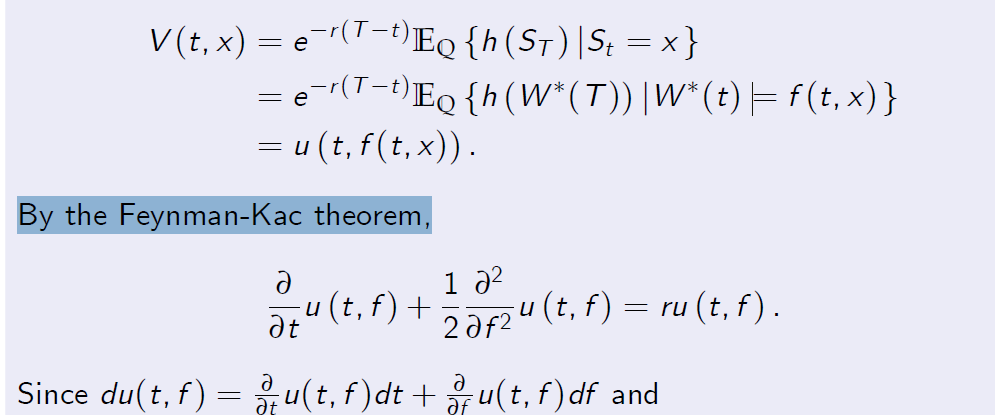
By the Feynman-Kac theorem,

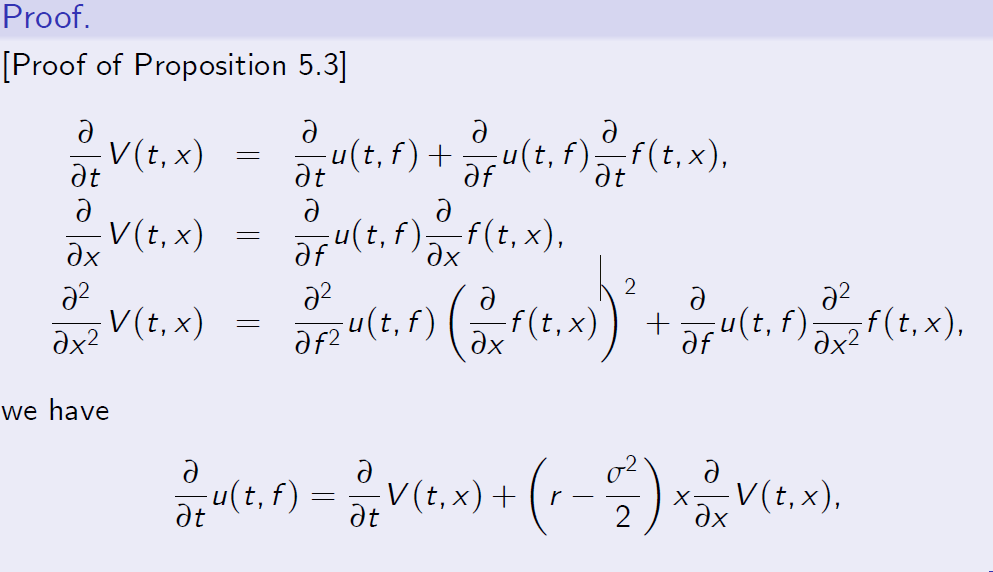
The Black-Scholes Model Proof. [Proof of Proposition 5.3]

The result follows from substituting them into the PDE for u(t, f ). Moreover, u (T, f (T, x)) = h(x) = V (t, x).

• To price a contingent claim under the Black-Scholes assumption, i.e., equation (1), one can either use the formula, equation (5), or solve the Black-Scholes equation.

Delta Hedging

• We create a riskless portfolio by buying a European option with strike price K and time to expiry T. The value of the option is C(S, t).

Suppose that a portfolio, with value \(\Pi\) consists of one option and a (negative) quantity \(-\Delta\) of the asset:
\(\Pi=C(S,t)-\Delta S\)

From the Ito formula the change in the prortfolio

Note that if \(\Delta = \frac {\partial C}{\partial S}\)then the risk is eliminated. The perfect elimination of risk is delta-hedging. Perfect hedge should be continuously rebalanced.

Delta Hedging

Choose \(\Delta = \frac {\partial C}{\partial S}\) and the resulting change in value is completely riskless:

it should be equal to the same return as if we invested in riskless interest-bearing account:

because of no arbitrage.

Which is the Black-Scholes equation.

Dividend-paying asset

Suppose the dividend yield is D. In a time dt each asset receives an anount DSdt. The value of portfolio

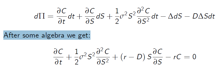
After some algebra we get:

Foreign currency

In holding the forign currency we receive interest at the foreign rate of interest \(r_f\) . This is like receiving a continuous dividend

Commodity Options

The storage of commodities is costly. Suppose q is the fraction of the value of a commodity that goes towards paying the cost of storage. For each unit of commodity held an amount qSdt will be required during time dt to finance the holding. This is like receiving a negative dividend.

Futures

The future price of a non-dividend paying equity F is related to the spot price by \(F = e^{r (T_F -t )}S\) where \(T_F\) is the maturity date of the futures contract. We can easily change variables and look for a solution C(S, t) = C(F, t). We find that

Black-Scholes Equation

To summarise, Black-Scholes equation is written in the form

where b is the cost-to-carry:

Asset with no dividend    b = r
Asset with dividend D    b = r - D
foreign currency with return \(r_f\)    \(b = r- r_f\)
Commodity with storage cost q    b = r + q
Futures    b = 0